Quasiparticle spectrum and dynamical stability of an atomic Bose-Einstein condensate coupled to a degenerate Fermi gas

Abstract

The quasiparticle excitations and dynamical stability of an atomic Bose-Einstein condensate coupled to a quantum degenerate Fermi gas of atoms at zero temperature is studied. The Fermi gas is assumed to be either in the normal state or to have undergone a phase transition to a superfluid state by forming Cooper pairs. The quasiparticle excitations of the Bose-Einstein condensate exhibit a dynamical instability due to a resonant exchange of energy and momentum with quasiparticle excitations of the Fermi gas. The stability regime for the bosons depends on whether the Fermi gas is in the normal state or in the superfluid state. We show that the energy gap in the quasiparticle spectrum for the superfluid state stabilizes the low energy energy excitations of the condensate. In the stable regime, we calculate the boson quasiparticle spectrum, which is modified by the fluctuations in the density of the Fermi gas.

I Introduction

Since the observation of Bose-Einstein condensation in trapped atomic gases BEC , there has been increasing interest in creating quantum degenerate gases of fermions with trapped ultracold akali atoms. At temperatures below the Fermi temperature, $T_{F}$, the properties of the gas become strongly influenced by the Pauli exclusion principle Pauli ; holland2 . Besides exploring the role of quantum statistics in their behavior, much of the interest in these gases has focused on the possibility of achieving the Bardeen-Cooper-Schrieffer (BCS) phase transition to the superfluid state by forming Cooper pairs Li6 ; burnett ; bohn ; holland ; mackie .

Currently, experimental efforts in cooling of fermionic atoms of ⁶Li truscott ; thomas and ⁴⁰K jin ; Pauli to the quantum degenerate regime have made significant progress, reaching temperatures as low as $0.2T_{F}$ where $T_{F}$ is the Fermi temperature. However, the efficiency of the evaporative cooling process used to cool a two component Fermi gas is severely hindered for temperatures below $T_{F}$ due to Pauli blocking holland2 . Meanwhile, the lack of $s$-wave scattering between spin-polarized fermions makes evaporative cooling completely ineffective for a single component Fermi gas. Furthermore, it has been recently predicted that loss processes which remove particles from the trap and leave holes behind in the single particle distribution also impose a lower limit on the temperature ($\sim T_{F}/4$) that can be reached in a pure Fermi gas eddy . As a result, the recent experiments that achieved quantum degeneracy in ⁶Li have used ⁷Li, a boson, to sympathetically cool the ⁶Li atoms truscott . This procedure is also being applied to cool ⁴⁰K using ⁸⁷Rb jin2 . Therefore, it appears likely that future experiments on degenerate Fermi gases will be associated with a Bose gas with a non-negligible boson-fermion two-body interaction. In a more speculative vein, the nonlinear mixing of bosonic and fermionic matter waves may open up the way to novel methods to manipulate these waves, and in particular their statistical properties. The theoretical study of the properties of coupled Bose-Einstein condensates and degenerate Fermi gases is therefore of considerable practical interest to future experiments.

It is the purpose of this paper to establish a general analysis of the quasiparticle spectrum and dynamical stability for a BEC coupled to a degenerate Fermi gas. There have been a number of recent studies of both the ground state properties molmer ; viverit ; roth ; yi and the collective modes for the density fluctuations of the coupled gases yip ; bijlsma ; capuzzi ; minguzzi1 . These studies have all treated the ground state of the fermions as being that of a normal degenerate Fermi gas. The likelihood of observing the superfluid state in fermionic akali vapors has sparked several theoretical studies of the quasiparticle and collective modes of trapped superfluid Fermi gases baranov ; minguzzi ; mottelson ; bruun . However, the quasiparticle excitations of a coupled superfluid Fermi gas and Bose-Einstein condensate (BEC) has not yet been investigated. In this paper, we examine both the case when the ground state of the fermions, in the absence of a boson-fermion interaction, is the normal state and the BCS superfluid state. In both cases, the quasiparticle spectrum exhibits a dynamical instability due to the exchange of energy and momentum with the fermions. Physically, the existence of the instability implies the existence of a lower energy ground state of the coupled system, which involves correlated density fluctuations between the BEC and Fermi gas. In the stable regime, the quasiparticle dispersion relation for the bosons is significantly modified due to quantum fluctuations in the density of the Fermi gas. More importantly, the stability regime and the quasiparticle dispersion for the bosons is qualitatively different when the fermions are in the BCS state as compared to the normal state.

In terms of current experiments with trapped atomic gases, we are only interested in the dilute limit for the Bose-Fermi mixture. In that limit, we can linearize the equations of motion for the density fluctuations of the two gases, since at zero temperature the fluctuations relative to the non-interacting ground state are expected to be small. For the bosons, this method is equivalent, in the absence of a boson-fermion coupling, to the Bogoliubov procedure bogo1 . The presence of a boson-fermion coupling results in a modified boson-boson interaction due to the induced density fluctuations in the Fermi gas. In Sec. II, we present our model and derive the quasiparticle spectrum for the bosons when the fermions are in the normal state. In Sec. III, we show how the calculation of Sec. II is modified when the fermions are in the BCS state. In the Appendix, we show how quantum correlations between the densities of the two gases can lower the ground state energy of the mixture.

II Mixture of BEC and Normal Fermi Gas

This paper focuses on the effect that the boson-fermion interaction has on the quasiparticles states of the Bose gas. Hence, we neglect the effect of a direct interaction between the fermions in this section. For a spin-polarized Fermi gas, this is an excellent approximation since $s$-wave scattering between two fermions is forbidden and $p$-wave scattering is negligible at zero temperature. However, for the sake of generality, we consider the case of fermions with two hyperfine spin states. The results of this section can be directly applied to a single component Fermi gas pu since we assume that the boson-fermion interaction and the single-particle energies of the fermions are independent of the spin. In the next section, we will generalize these results to the case of $s$-wave Cooper pairing. For this purpose, it will be necessary to explicitly include an attractive interaction in order to create a non-zero pairing field needed for the BCS state.

Our starting point is the grand canonical Hamiltonian for a weakly interacting gas of bosons coupled to an ideal gas of fermions with the two spin states, labelled by $\sigma=\uparrow,\downarrow$,

$$\hat{H}=\hat{H}_{B}+\hat{H}_{F}+\hat{H}_{BF},$$ (1)

where $\hat{H}_{B}$ and $\hat{H}_{F}$ are the free Hamiltonians for the bosons and fermions, respectively,

$$\hat{H}_{B} = \int d^{3}r\,\hat{\psi}^{\dagger}_{B}({\bf r})\left[-\frac{\hbar^{2}\nabla^{2}}{2m_{B}}+V_{B}({\bf r})-\mu_{B}\right.$$

$$\left.+\frac{g_{B}}{2}\hat{\psi}^{\dagger}_{B}({\bf r})\hat{\psi}_{B}({\bf r})\right]\hat{\psi}_{B}({\bf r}),$$

$$\hat{H}_{F} = \sum_{\sigma}\int d^{3}r\,\hat{\psi}^{\dagger}_{\sigma}({\bf r})\left[-\frac{\hbar^{2}\nabla^{2}}{2m_{F}}+V_{F}({\bf r})-\mu_{\sigma}\right]\hat{\psi}_{\sigma}({\bf r}),$$

while $\hat{H}_{BF}$ represents the boson-fermion interaction,

$$\hat{H}_{BF}=g_{BF}\sum_{\sigma}\int d^{3}r\,\hat{\psi}^{\dagger}_{B}({\bf r})\hat{\psi}^{\dagger}_{\sigma}({\bf r})\hat{\psi}_{\sigma}({\bf r})\hat{\psi}_{B}({\bf r}).$$

Here, $\hat{\psi}_{B}({\bf r})$ $[\hat{\psi}^{\dagger}_{B}({\bf r})]$ and $\hat{\psi}_{\sigma}({\bf r})$ $[\hat{\psi}^{\dagger}_{\sigma}({\bf r})]$ are the annihilation (creation) operators for the bosons and for fermions with hyperfine spin $\sigma$, respectively. They obey the standard commutation (anti-commutation) relations. $\mu_{B}$ and $\mu_{\sigma}$ are the chemical potentials for the bosons and fermions. The coupling constants, $g_{B}$ and $g_{BF}$, are defined as

$$g_{B}=4\pi\hbar^{2}a_{B}/m_{B},\;\;g_{BF}=2\pi\hbar^{2}a_{BF}/m_{r},$$

where $a_{B}>0$ and $a_{BF}$ are the boson-boson and boson-fermion $s$-wave scattering lengths, respectively, while $m_{r}=m_{B}m_{F}/(m_{B}+m_{F})$ is the reduced mass. For simplicity, we assume that the number of fermions in each spin state is the same so that $\mu_{\uparrow,\downarrow}=\mu_{F}$.

To determine the excitation spectrum of the Bose-condensate, we apply the standard Bogoliubov procedure by decomposing the field operator as

$$\hat{\psi}_{B}({\bf r},t)=\phi_{B}({\bf r})+\hat{\xi}_{B}({\bf r},t).$$ (2)

Here, $\hat{\xi}_{B}({\bf r},t)$ describes the small amplitude fluctuations above the condensate mode, $\phi_{B}({\bf r})$, which obeys the Gross-Pitaevskii equation,

$$\left[-\frac{\hbar^{2}\nabla^{2}}{2m_{B}}+V_{B}({\bf r})+g_{B}|\phi_{B}({\bf r})|^{2}+2g_{BF}n_{F}({\bf r})-\mu_{B}\right]$$ (3)

$$\times\phi_{B}({\bf r})=0.$$

Similarly, we assume that the density fluctuations in the Fermi gas are small so that

$$\hat{\psi}_{\sigma}^{\dagger}({\bf r},t)\hat{\psi}_{\sigma}({\bf r},t)=n_{F}({\bf r})+\delta\hat{\rho}_{\sigma}({\bf r},t)$$ (4)

where $\langle\delta\hat{\rho}_{\sigma}({\bf r},t)\rangle=0$ in the absence of any external perturbations. For a trapped gas, the equilibrium density of each spin component, $n_{F}({\bf r})$, may be approximated by the Thomas-Fermi expression for the density molmer . There is an obvious asymmetry in our treatment of the bosons and fermions since for the BEC there is a nonvanishing expectation of $\hat{\psi}_{B}({\bf r},t)$ while for the fermions, $\langle\hat{\psi}_{\sigma}({\bf r},t)\rangle=0$ and only the fluctuations in the fermion density may be regarded as being small relative to some finite mean-field.

By substituting Eqs. (2) and (4) into Eq. (1), and neglecting terms involving the product of three or more fluctuation operators, one obtains a Hamiltonian that is quadratic in $\hat{\xi}_{B}({\bf r},t)$ and $\hat{\psi}_{\sigma}({\bf r})$. From this quadratic Hamiltonian, one obtains Heisenberg equations of motion that are linear in the fluctuations,

$$i\hbar\frac{\partial\hat{\xi}_{B}}{\partial t} = \hat{h}_{B}\hat{\xi}_{B}+g_{B}\phi_{B}^{2}\hat{\xi}_{B}^{\dagger}+g_{BF}\phi_{B}\sum_{\sigma}\delta\hat{\rho}_{\sigma},$$ (5)

$$i\hbar\frac{\partial\hat{\psi}_{\sigma}}{\partial t} = \hat{h}_{F}\hat{\psi}_{\sigma}+g_{BF}(\phi_{B}\hat{\xi}_{B}^{\dagger}+\phi_{B}^{*}\hat{\xi}_{B})\hat{\psi}_{\sigma},$$ (6)

where

$$\hat{h}_{B} = -\frac{\hbar^{2}\nabla^{2}}{2m_{B}}+V_{B}({\bf r})+2g_{B}|\phi_{B}({\bf r})|^{2}+2g_{BF}n_{F}({\bf r})-\mu_{B},$$

$$\hat{h}_{F} = -\frac{\hbar^{2}\nabla^{2}}{2m_{F}}+V_{F}({\bf r})+g_{BF}|\phi_{B}({\bf r})|^{2}-\mu_{F}.$$

Equations (5) and (6) can be thought of as describing a four-wave mixing process where a bosonic wave, $\phi_{B}({\bf r})$, scatters off the fermionic density grating, $\delta\hat{\rho}_{\sigma}$, to create a new bosonic wave, $\hat{{\xi}_{B}}({\bf r},t)$. Equation (6) represents the back-action on the fermion grating as a result of the scattering of the bosonic wave. In contrast to Ref.moore , where the fermionic grating was created optically, or matter-wave superradiance superrad , where the grating results from the mixing of optical and matter waves, four-wave mixing results now from the coupling between the bosonic and fermionic matter-wave fields.

The procedure we adopt here is to formally integrate Eq. (6) to obtain a linearized expression for $\delta\hat{\rho}_{\sigma}$, which can then be substituted back into Eq. (5) to obtain an integro-differential equation for the boson fluctuation operators. To begin, we expand the fermion field operators in terms of the eigenstates of $\hat{h}_{F}$,

$$\hat{\psi}_{\sigma}({\bf r},t)=\sum_{n}\,\hat{a}_{n,\sigma}(t)\varphi_{n}({\bf r}),$$ (7)

where $\hat{h}_{F}\varphi_{n}({\bf r})=E_{n}\varphi_{n}({\bf r})$. The formal solution of Eq. (6) is then given by

$$\hat{\psi}_{\sigma}({\bf r},t) = \hat{\psi}_{\sigma}^{(0)}({\bf r},t)-i\frac{g_{BF}}{\hbar}\int_{0}^{t}dt^{\prime}\int d^{3}r^{\prime}\,G({\bf r},{\bf r^{\prime}},t-t^{\prime})$$ (8)

$$\;\;\times\,\Xi({\bf r^{\prime}},t^{\prime})\hat{\psi}_{\sigma}({\bf r^{\prime}},t^{\prime}),$$

where

$$\hat{\psi}_{\sigma}^{(0)}({\bf r},t)=\sum_{n}\hat{a}_{n,\sigma}(0)e^{-iE_{n}t/\hbar}\varphi_{n}({\bf r})$$ (9)

represents the free evolution of the field in the absence of a density fluctuation of the BEC, and

$$\Xi({\bf r},t)=\phi_{B}({\bf r})\hat{\xi}_{B}^{\dagger}({\bf r},t)+\phi_{B}^{*}({\bf r})\hat{\xi}_{B}({\bf r},t).$$ (10)

Physically, $\Xi({\bf r},t)$ produces a density grating off which the fermions can scatter. Consequently, the second term on the right hand side of Eq. (8) may be interpreted as the scattering of the fermions off the potential $g_{BF}\Xi({\bf r^{\prime}},t^{\prime})$ and the subsequent propagation of the fermions to $({\bf r},t)$ by the single particle Green’s function,

$$G({\bf r},{\bf r^{\prime}},t-t^{\prime})\equiv\sum_{n}e^{-iE_{n}(t-t^{\prime})/\hbar}\varphi_{n}({\bf r})\varphi_{n}^{*}({\bf r^{\prime}}).$$ (11)

In order to obtain a linear equation for the boson fluctuations, we make the first Born approximation in Eq. (8), so that

$$\hat{\psi}_{\sigma}({\bf r},t) \approx \hat{\psi}_{\sigma}^{(0)}({\bf r},t)-i\frac{g_{BF}}{\hbar}\int_{0}^{t}dt^{\prime}\int d^{3}r^{\prime}\,G({\bf r},{\bf r^{\prime}},t-t^{\prime})$$ (12)

$$\;\;\times\,\Xi({\bf r^{\prime}},t^{\prime})\hat{\psi}_{\sigma}^{(0)}({\bf r^{\prime}},t^{\prime}).$$

An expression for the fermion density fluctuation that is linear in the boson fluctuations is obtained from Eq. (12) and

$$\delta\hat{\rho}_{\sigma}=\langle F|\hat{\psi}_{\sigma}^{\dagger}({\bf r},t)\hat{\psi}_{\sigma}({\bf r},t)|F\rangle-n_{F}({\bf r}),$$ (13)

where $|F\rangle$ represents the zero temperature ground state of the Fermi gas. By making use of the fact that at $T=0$, $\langle F|\hat{a}^{\dagger}_{n,\sigma}(0)\hat{a}_{n^{\prime},\sigma^{\prime}}(0)|F\rangle=\delta_{n,n^{\prime}}\delta_{\sigma,\sigma^{\prime}}$ for $E_{n}\leq E_{F}$ and zero otherwise ($E_{F}$ is the Fermi energy) as well as $\sum_{n}|\varphi_{n}({\bf r})|^{2}=n_{F}({\bf r})$, we obtain the desired expression for the fermion density fluctuation due to the coupling to the bosons,

$$\delta\hat{\rho}_{\sigma}\approx i\frac{g_{BF}}{\hbar}\int_{0}^{t}dt^{\prime}\int d^{3}r^{\prime}\,{\cal J}({\bf r},{\bf r^{\prime}},t-t^{\prime})\Xi({\bf r^{\prime}},t^{\prime}),$$ (14)

where

$${\cal J}({\bf r},{\bf r^{\prime}},t-t^{\prime}) \equiv G^{*}_{>}({\bf r},{\bf r^{\prime}},t-t^{\prime})G_{<}({\bf r},{\bf r^{\prime}},t-t^{\prime})$$

$$\;-G_{>}({\bf r},{\bf r^{\prime}},t-t^{\prime})G_{<}^{*}({\bf r},{\bf r^{\prime}},t-t^{\prime}),$$

$$G_{>}({\bf r},{\bf r^{\prime}},t-t^{\prime}) \equiv \sum_{\{n|E_{n}>E_{F}\}}e^{-iE_{n}(t-t^{\prime})/\hbar}\varphi^{*}_{n}({\bf r^{\prime}})\varphi_{n}({\bf r}),$$

and $G_{<}$ is the same as $G_{>}$, but for $E_{n}\leq E_{F}$ in the summation. By inserting Eq. (14) back into Eq. (5) we finally have

$$i\hbar\frac{\partial\hat{\xi}_{B}({\bf r},t)}{\partial t}=\hat{h}_{B}\hat{\xi}_{B}({\bf r},t)+g_{B}\phi_{B}^{2}\hat{\xi}_{B}^{\dagger}({\bf r},t)+i\frac{2g_{BF}^{2}}{\hbar}\int_{0}^{t}dt^{\prime}\int d^{3}r^{\prime}\,{\cal J}({\bf r},{\bf r^{\prime}},t-t^{\prime})\Xi({\bf r^{\prime}},t^{\prime})\phi_{B}({\bf r}).$$ (15)

Equation (15) is valid to all orders in $g_{BF}$ provided the density fluctuations of the bosons, $\Xi({\bf r},t)$, and the fermions, $\delta\hat{\rho}_{\sigma}({\bf r},t)$, remain small relative to the equilibrium densities of the two gases. The dependence of $\hat{\xi}_{B}$ to all orders in $g_{BF}$ is easily seen by iterating the expression for $\Xi({\bf r},t)$ inside the integrand to obtain a power series expansion in even powers of $g_{BF}$.

The physical interpretation of the integral term in Eq. (15) is straightforward. Since the boson-fermion interaction is proportional to the local densities of the two gases, a density fluctuation in the BEC at ${\bf r^{\prime}}$ and $t^{\prime}$, $\Xi({\bf r^{\prime}},t^{\prime})$, will excite a density fluctuation in the Fermi gas at the same point. This density fluctuation consists of particles excited above the Fermi surface, which are represented by $G_{>}$, and holes inside the Fermi sea, represented by $G_{<}$. These particle-hole pairs then propagate from ${\bf r^{\prime}}$ and $t^{\prime}$ to ${\bf r}$ and $t$ where they excite another fluctuation in the density of the BEC, thereby modifying the value of $\hat{\xi}_{B}({\bf r},t)$ and hence, $\Xi({\bf r},t)$. The integral in Eq. (15) may then be thought of as a feedback loop where the density fluctuations of the Fermi gas act as the feedback mechanism. If the BEC is stable, the feedback will be negative while for an unstable system, the coupled boson-fermion density fluctuations will result in a positive feedback, which causes the fluctuations to grow exponentially in time.

Equation (15), which is the main result of this section, is completely general. However, for concreteness, we consider a homogenous mixture of $N_{B}$ bosons and $2N_{F}$ fermions confined in a box of volume $V$. The corresponding ground state densities are $n_{B}=|\phi({\bf r})|^{2}=N_{B}/V$ and $n_{F}=n_{F}({\bf r})=N_{F}/V$. The chemical potentials are $\mu_{B}=g_{B}n_{B}+2g_{BF}n_{F}$ [see Eq. (3)] and $E_{F}=\hbar^{2}k_{F}^{2}/2m_{F}=\mu_{F}-g_{BF}n_{B}$ where the Fermi wave number is given by $k_{F}=[(6\pi^{2})n_{F}]^{1/3}$. For periodic boundary conditions, the eigenstates of $\hat{h}_{F}$ are plane waves $\varphi_{{\bf k}}({\bf r})=e^{i{\bf k\cdot r}}/\sqrt{V}$ with eigenenergies $E_{{\bf k}}=\hbar^{2}k^{2}/2m_{F}-E_{F}$. Similarly, we use a plane wave basis for the boson field operator,

$$\hat{\psi}_{B}({\bf r},t)=\frac{1}{\sqrt{V}}\sum_{{\bf k}}\eta_{{\bf k}}(t)e^{i{\bf k}\cdot{\bf r}}\,.$$ (16)

Hence, the boson fluctuation operator consists of all modes with ${\bf k}\neq 0$,

$$\hat{\xi}_{B}({\bf r},t)=\frac{1}{\sqrt{V}}\sum_{{\bf k}\neq 0}\eta_{{\bf k}}(t)e^{i{\bf k}\cdot{\bf r}}\,.$$ (17)

The quantum state of the mixture can therefore be expressed as

$$|\Psi_{N}\rangle=\frac{1}{\sqrt{N_{B}!}}\left(\eta^{\dagger}_{0}\right)^{N_{B}}\prod_{k\leq k_{F},\sigma}a^{\dagger}_{{\bf k}\sigma}|0\rangle,$$ (18)

where $|0\rangle$ represents the vacuum state for both the bosons and fermions. Note that $|\Psi_{N}\rangle$ is identical to the state assumed by Viverit et al. viverit , if one includes two spin components.

The function ${\cal J}({\bf r},{\bf r^{\prime}},t-t^{\prime})$, which describes the propagation of particle-hole pairs in the Fermi gas, can now be expressed explicitly as

$${\cal J}({\bf r},{\bf r^{\prime}},t-t^{\prime})= \frac{1}{V^{2}} \sum_{k_{n}>k_{F}}\sum_{k_{m}\leq k_{F}}\left[e^{i\frac{\hbar}{2m_{F}}(k_{n}^{2}-k_{m}^{2})(t-t^{\prime})}\right.$$

$$\times\left.e^{i({\bf k_{m}}-{\bf k_{n}})\cdot{\bf r}}e^{-i({\bf k_{m}}-{\bf k_{n}})\cdot{\bf r^{\prime}}}-c.c.\right].$$

Multiplying Eq. (15) by $e^{-i{\bf k\cdot r}}/\sqrt{V}$ and integrating over ${\bf r}$ one obtains

$$i\hbar\frac{\partial\eta_{{\bf k}}}{\partial t}={\cal L}_{B}(k)\eta_{{\bf k}}+g_{B}n_{B}\eta_{-{\bf k}}^{\dagger}+\frac{i}{\hbar}g_{BF}^{2}n_{B}I({\bf k}),$$ (19)

where ${\cal L}_{B}(k)=\hbar^{2}k^{2}/2m_{B}+g_{B}n_{B}$, and

$$I({\bf k}) = \frac{2}{V}\int_{0}^{t}dt^{\prime}\int d^{3}r^{\prime}\int d^{3}r\,e^{-i{\bf k}\cdot{\bf r}}{\cal J}({\bf r},{\bf r^{\prime}},t-t^{\prime})\,\sum_{{\bf k^{\prime}}}e^{i{\bf k^{\prime}}\cdot{\bf r^{\prime}}}\left[\eta^{\dagger}_{-{\bf k^{\prime}}}(t^{\prime})+\eta_{{\bf k^{\prime}}}(t^{\prime})\right]$$

$$= \frac{2}{V}\int_{0}^{t}dt^{\prime}\,\sum_{k_{m}\leq k_{F}}\left[e^{i\frac{\hbar}{2m_{F}}(|{\bf k_{m}}+{\bf k}|^{2}-k_{m}^{2})(t-t^{\prime})}-c.c.\right]\,\Theta(|{\bf k_{m}}+{\bf k}|-k_{F})\left[\eta^{\dagger}_{-{\bf k}}(t^{\prime})+\eta_{{\bf k}}(t^{\prime})\right],$$

where $\Theta(x)$ is the unit step function. By taking the adjoint of Eq. (19) and using $I^{\dagger}(-{\bf k})=-I({\bf k})$ one gets,

$$i\hbar\frac{\partial\eta^{\dagger}_{-{\bf k}}}{\partial t}=-{\cal L}_{B}(k)\eta^{\dagger}_{-{\bf k}}-g_{B}n_{B}\eta_{{\bf k}}-\frac{i}{\hbar}g_{BF}^{2}n_{B}I({\bf k}).$$ (20)

The coupled integro-differential Eqs. (19) and (20) may be solved using Laplace transforms. Denoting the single-sided Laplace transforms as,

$$\alpha_{{\bf k}}(s) = L[\eta_{{\bf k}}(t)]=\int^{\infty}_{0}dt\,e^{-st}\eta_{{\bf k}}(t),$$

$$\beta_{{\bf k}}(s) = L[\eta^{\dagger}_{-{\bf k}}(t)]=\int^{\infty}_{0}dt\,e^{-st}\eta^{\dagger}_{-{\bf k}}(t),$$

one obtains the inhomogeneous linear equations

$$i\hbar[s\alpha_{{\bf k}}(s)-\eta_{{\bf k}}(0)] = {\cal L}_{B}(k)\alpha_{{\bf k}}(s)+g_{B}n_{B}\beta_{{\bf k}}(s)+\frac{g_{BF}^{2}}{\hbar(2\pi)^{3}}n_{B}\ell_{k}(s)[\alpha_{{\bf k}}(s)+\beta_{{\bf k}}(s)],$$ (21a)

$$i\hbar[s\beta_{{\bf k}}(s)-\eta^{\dagger}_{-{\bf k}}(0)] = -{\cal L}_{B}(k)\beta_{{\bf k}}(s)-g_{B}n_{B}\alpha_{{\bf k}}(s)-\frac{g_{BF}^{2}}{\hbar(2\pi)^{3}}n_{B}\ell_{k}(s)[\alpha_{{\bf k}}(s)+\beta_{{\bf k}}(s)],$$ (21b)

where

$$\ell_{k}(s) = \frac{2i(2\pi)^{3}}{V}L\left[\sum_{k_{m}\leq k_{F}}^{|{\bf k_{m}}+{\bf k}|>k_{F}}e^{i(|E_{{\bf k+k_{m}}}|+|E_{{\bf k_{m}}}|)t/\hbar}-c.c.\right]$$

$$= 2\int d{\bf k_{m}}\left[\frac{1}{-is-(|E_{{\bf k+k_{m}}}|+|E_{{\bf k_{m}}}|)/\hbar}-\frac{1}{-is+(|E_{{\bf k+k_{m}}}|+|E_{{\bf k_{m}}}|)/\hbar}\right]\Theta(|{\bf k_{m}}+{\bf k}|-k_{F})\Theta(k_{F}-k_{m}).$$

and in the second line we have taken the infinite volume limit to convert the summation to an integral. The solutions of Eqs. (21) are,

$$\alpha_{{\bf k}}(s) = i\hbar\frac{\left[\zeta_{k}(s)+\left(i\hbar s+T_{k}\right)\eta_{{\bf k}}(0)\right]}{(i\hbar s)^{2}-z_{k}(s)}\,,$$ (23a)

$$\beta_{{\bf k}}(s) = i\hbar\frac{\left[-\zeta_{k}(s)+\left(i\hbar s-T_{k}\right)\eta^{\dagger}_{-{\bf k}}(0)\right]}{(i\hbar s)^{2}-z_{k}(s)}\,,$$ (23b)

where $T_{k}=\hbar^{2}k^{2}/(2m_{B})$ and

$$\zeta_{k}(s) = n_{B}\left[g_{B}+\frac{g_{BF}^{2}\ell_{k}(s)}{\hbar(2\pi)^{3}}\right]\left[\eta_{{\bf k}}(0)+\eta^{\dagger}_{-{\bf k}}(0)\right],$$

$$z_{k}(s) = T_{k}\left[T_{k}+2n_{B}\left(g_{B}+\frac{g_{BF}^{2}}{\hbar(2\pi)^{3}}\ell_{k}(s)\right)\right].$$

The poles of Eqs. (23) in the $s$-plane correspond to the quasiparticle excitation frequencies of the condensate. For $g_{BF}=0$, one obviously recovers the Bogoliubov spectrum of a pure weakly interacting BEC. For $s=i\omega+0^{+}$, $\ell_{k}(s)$ is proportional to the density-density response function of an ideal Fermi gas, which measures the linear response of the density of the gas to a scalar perturbing potential pines . The expression $g_{B}+g_{BF}^{2}\ell_{k}(s)/\hbar(2\pi)^{3}$ corresponds to a renormalized boson-boson interaction due to the polarization of the density of the Fermi gas.

We already mentioned that in case of positive feedback between the density fluctuations in the two gases, the BEC becomes unstable. Mathematically, the stability of the BEC is determined by the location of the poles in the $s$-plane,

$$(i\hbar s)^{2}-z_{k}(s)=0.$$ (24)

In order for the BEC to be stable, Re$[s]<0$ for all solutions of (24). A positive real part of any of the poles indicates the existence of an instability in the BEC.

To evaluate the boson excitation frequencies in the stable regime as well as the location of the instabilities it is sufficient to make the substitution $s=i\omega+0^{+}$, in which case the condition that the BEC be stable corresponds to poles with Im$[\omega]>0$. The real and imaginary parts of $\ell_{k}(\omega)\equiv\ell_{k}(s=i\omega+0^{+})$ can be obtained using $1/(x\pm i0^{+})=P(1/x)\mp i\pi\delta(x)$ fetter ,

$${\rm Re}[\ell_{k}(\omega)] = \frac{2\pi}{\alpha}\left\{\left[k_{F}^{2}-\left(\frac{\omega}{\alpha}-\frac{k}{2}\right)^{2}\right]\ln\left|\frac{\omega+\alpha(k_{F}-k/2)}{\omega-\alpha(k_{F}+k/2)}\right|+\left[k_{F}^{2}-\left(\frac{\omega}{\alpha}+\frac{k}{2}\right)^{2}\right]\ln\left|\frac{\omega-\alpha(k_{F}-k/2)}{\omega+\alpha(k_{F}+k/2)}\right|-2k_{F}k\right\},$$

$${\rm Im}[\ell_{k}(\omega)] = 2\pi\int d{\bf k_{m}}\,\Theta(|{\bf k_{m}}+{\bf k}|-k_{F})\Theta(k_{F}-k_{m})\times\,\delta\left(\omega-|E_{{\bf k_{m}}+{\bf k}}|/\hbar-|E_{{\bf k_{m}}}|/\hbar\right),$$ (25)

where $\alpha=\hbar k/m_{F}$.

The mechanical stability of the condensate, which requires its compressibility to be positive, can be derived from the zero frequency ($\omega=0$) static limit for the speed of sound in the condensate. From Eq. (24), in the long wavelength limit (i.e., $k\rightarrow 0$), we have $\omega^{2}=c_{B}^{2}k^{2}$ where $c_{B}$ is the speed of sound. A positive compressibility corresponds to $c_{B}^{2}\geq 0$. From Eq. (24), $c_{B}^{2}$ is given by,

$$c_{B}^{2}=\frac{n_{B}}{m_{B}}\left[g_{B}+\frac{g_{BF}^{2}}{\hbar(2\pi)^{3}}\lim_{k\rightarrow 0}\ell_{k}(0)\right].$$ (26)

Using the expansion of $\ell_{k}(0)$ for $k\ll k_{F}$,

$$\ell_{k}(0)\approx\frac{4\pi m_{F}k_{F}}{\hbar}\left[-2+\frac{1}{6}\left(\frac{k}{k_{F}}\right)^{2}\right],$$ (27)

one obtains the mechanical stability condition,

$$n_{F}^{1/3}\leq\frac{A}{3}\frac{g_{B}}{g_{BF}^{2}}\,,$$ (28)

where $A=(\hbar^{2}/2m_{F})(6\pi^{2})^{2/3}$, or in terms of scattering lengths,

$$a_{BF}^{2}\leq\frac{\pi a_{B}m_{B}m_{F}}{k_{F}(m_{B}+m_{F})^{2}}.$$

Eq. (28) agrees with the result obtained in Refs. viverit ; yip ; bijlsma when one accounts for the two spin components. In the following it will be assumed that Eq. (28) is satisfied.

A necessary condition for the BEC to be dynamically stable with respect to density fluctuations of finite energy and momentum is that ${\rm Im}[\ell_{k}(\omega)]=0$. Since ${\rm Im}[\ell_{k}(\omega)]$ is proportional to the dynamic structure factor of the Fermi gas, it measures the rate at which energy and momentum can be resonantly transferred between the density fluctuations in the Fermi and Bose gases pines . In the absence of any decay or dephasing mechanism for the boson or fermion quasiparticles, the existence of a bosonic quasiparticle with energy $\hbar{\rm Re}[\omega({\bf k})]$ such that ${\rm Im}[\ell_{k}(\omega)]\neq 0$ will give rise to coupled oscillations between the density fluctuations with wave vector ${\bf k}$, similar to Rabi oscillations for a two-level atom coupled to a quantized field meystre . One may then consider a new ground state, which is a superposition of a bosonic and fermionic density fluctuation, in analogy to the dressed states of quantum optics meystre . In the appendix it is shown that such a superposition can result in a state with an energy lower than the state used in this section and in other studies of Bose-Fermi mixtures molmer ; viverit ; roth ; yi ; yip ; bijlsma ; capuzzi ; minguzzi , which do not contain any quantum correlations between the densities of the two gases. This indicates that a dynamical instability signified by ${\rm Im}[\ell_{k}(\omega)]\neq 0$ leads to a lower energy ground state of the Bose-Fermi mixture. It is worth noting that the dynamical instability is distinct from the mechanical instability of the mixture, discussed previously. A mechanical instability due to the Bose-Fermi coupling leads to a demixing of the two gases and occurs in the static ($\omega=0$) limit for which ${\rm Im}[\ell_{k}(\omega)]$ is always zero.

For excitations of the BEC with frequency $\omega$ and wave number $k<2k_{F}$, the stability criterion determined by ${\rm Im}[\ell_{k}(\omega)]=0$ requires the excitation frequency to satisfy

$$\omega>\frac{\hbar k^{2}}{2m_{F}}+\frac{\hbar kk_{F}}{m_{F}}.$$ (29)

Physically, $\hbar^{2}k^{2}/2m_{F}+\hbar^{2}kk_{F}/m_{F}$ is the maximum energy that a particle-hole pair can have for a given $k$. Hence, the stability criterion corresponds to there being no excitations of the Fermi gas that can resonantly couple to the condensate quasiparticle.

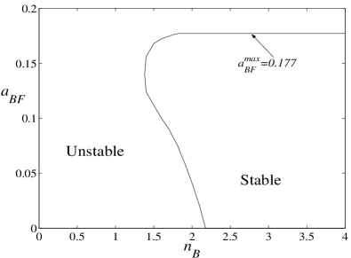
Figure 1: Stability diagram of a Bose-Fermi mixture. We assume $m_{F}=m_{B}=m$. We have adopted a system of units in which the units for frequency, length, and wavenumber are $\hbar k_{F}^{2}/2m$, $1/k_{F}$, and $k_{F}$, respectively. Note that in this units, the fermion density is given by $n_{F}=1/(6\pi^{2})\approx 0.017$.

The stability regime and the phonon spectrum can be obtained by first solving

$$(\hbar\omega)^{2} = z_{k}(i\omega+0^{+})$$ (30)

$$= T_{k}\left[T_{k}+2n_{B}\left(g_{B}+\frac{g_{BF}^{2}}{\hbar(2\pi)^{3}}{\rm Re}[\ell_{k}(\omega)]\right)\right],$$

numerically while assuming Im$[\ell_{k}(\omega)]=0$, and then checking if the system is stable using the criterion (29). Fig. 1 shows the stability diagram of the mixture in the $a_{BF}-n_{B}$ space. As can be seen, the dynamical stability of the system is determined by both the scattering lengths and the atomic densities. All other parameters being fixed, the stability condition (29) imposes a minimum boson density $n_{B}^{min}$ beyond which no stable homogeneous mixture exists. For $k\ll k_{F}$, we can use the linear part of the Bogoliubov spectrum for a pure condensate to estimate $n_{B}^{min}$ as

$$gn_{B}^{min}\approx\frac{\hbar^{2}k_{F}^{2}}{m_{F}^{2}/m_{B}}=\frac{\hbar^{2}(6\pi^{2}n_{F})^{2/3}}{m_{F}^{2}/m_{B}}.$$

For realistic numbers, $n_{B}^{min}$ is about two orders of magnitude larger than $n_{F}$ (see Fig. 1).

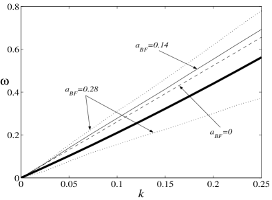
Figure 2: Phonon spectrum of a boson-fermion mixture. The thick solid line corresponds to $\omega=\hbar(k^{2}+2kk_{F})/2m_{F}$. Frequencies fall below this line represent unstable excitations. Same units as in Fig. 1.

Figure 2 illustrates the phonon spectrum for the BEC in the Bose-Fermi mixture when $n_{B}>n_{B}^{min}$. The boson-fermion interaction increases the sound velocity of the phonons. This effect has a straightforward explanation in terms of the stability condition imposed on the boson quasiparticle excitation frequency. In the stable regime determined by (29), the density-density response function $\ell_{k}(\omega)$ can be easily shown to be positive, hence $\omega(k)$, as given by Eq. (30), is increased.

For small values of $a_{BF}$, the spectrum is stable and single-valued. By expanding $\ell_{k}(\omega)$ around small $k/k_{F}$ and finite $\omega$, we can calculate the sound velocity, $c$, in the condensate for finite $\omega$ and $k$. Expanding $\ell_{k}(\omega)$ to lowest order in $k/k_{F}$, we obtain $\ell_{k}(\omega)=(8\pi\hbar/3)(k_{F}^{3}k^{2}/m_{F}\omega^{2})$, and hence the sound velocity is

$$c\approx c_{0}\left[1+\frac{g_{BF}^{2}k_{F}^{3}}{3\pi^{2}g_{B}m_{F}c_{0}^{2}}\right],$$ (31)

where $c_{0}=\sqrt{g_{B}n_{B}/m_{B}}$ is the sound velocity in a pure condensate. For the parameters in Fig. 2, we have a 6% increase in sound velocity if $a_{BF}$ changes from 0 to 0.14. However, further increasing $a_{BF}$ beyond a critical value $a_{BF}^{max}$ splits the phonon spectrum into two branches, and one of them falls into the unstable regime. The critical value of $a_{BF}$ for which the spectrum splits into two branches corresponds to the equality in Eq. (28). For $m_{F}\approx m_{B}$, we have $a_{BF}^{max}=\sqrt{\pi a_{B}/k_{F}}/2$, which gives the maximum sound velocity achievable in a homogeneous mixture

$$c_{max}=c_{0}\left(1+\frac{c_{F}^{2}}{c_{0}^{2}}\right),$$

where $c_{F}=\hbar k_{F}/(\sqrt{3}m_{F})$ is sound velocity of the ideal Fermi gas fetter . Note that while $n_{B}^{min}$ is independent of $a_{BF}$, $a_{BF}^{max}$ is independent of $n_{B}$.

III Mixture of BEC and Superfluid Fermi Gas

In order for a BCS transition to occur in a system of fermions, there must be an attractive two-body interaction which allows the fermions to form Cooper pairs. At the ultracold temperatures achieved in current experiments, $p$-wave collisions between atoms are highly suppressed and $s$-wave collisions between atoms in the same internal state are forbidden by the Pauli exclusion principle. As a result, the most likely possibility for the formation of Cooper pairs is an attractive $s$-wave interaction between atoms in different hyperfine states. Fortunately, ⁶Li and ⁴⁰K appear to be very promising candidates. ⁶Li possesses an anomalously large and negative $s$-wave scattering length, $a=-2160a_{B}$ where $a_{B}$ is the Bohr radius Li6 . For ⁴⁰K, a Feshbach resonance exists for two of the hyperfine states which can be used to create a large negative scattering length of $a\approx-1000a_{B}$ bohn . To deal with this situation, we now include in Eq. (1) the term

$$\hat{H}_{FF}=-g_{F}\int d^{3}r\,\hat{\psi}^{\dagger}_{\uparrow}({\bf r})\hat{\psi}^{\dagger}_{\downarrow}({\bf r})\hat{\psi}_{\downarrow}({\bf r})\hat{\psi}_{\uparrow}({\bf r}),$$ (32)

where $g_{F}=4\pi\hbar^{2}|a_{F}|/m_{F}$ and $a_{F}<0$ is the $s$-wave scattering length between fermions in the spin singlet state. $\hat{H}_{FF}$ can be treated using the self-consistent field method by replacing pairs of fermion operators in $\hat{H}_{FF}$ with $c$-numbers degennes ,

$$\hat{H}_{FF} = \int d^{3}r\left[-g_{F}n_{F}({\bf r})\sum_{\sigma}\hat{\psi}^{\dagger}_{\sigma}({\bf r})\hat{\psi}_{\sigma}({\bf r})\right.$$ (33)

$$\left.+\Delta({\bf r})\hat{\psi}^{\dagger}_{\uparrow}({\bf r})\hat{\psi}^{\dagger}_{\downarrow}({\bf r})+\Delta^{*}({\bf r})\hat{\psi}_{\downarrow}({\bf r})\hat{\psi}_{\uparrow}({\bf r})\right],$$

where

$$\Delta({\bf r})=-g_{F}\langle\hat{\psi}_{\downarrow}({\bf r})\hat{\psi}_{\uparrow}({\bf r})\rangle,$$ (34)

and the expectation value is taken with respect to the BCS ground state defined below. $\Delta({\bf r})$ is the order parameter for the BCS state. It represents the correlation between fermions that have formed Cooper pairs and is zero for the normal state of the Fermi gas. The term proportional to $-g_{F}n_{F}({\bf r})$, is a Hartree-Fock mean-field which is present even in the normal state for an interacting Fermi gas. The inclusion of a Hartree-Fock term for the normal state does not affect any of the results of the last section since, in particular for a uniform system, it can be absorbed into the definition of the Fermi energy.

We now proceed as before and calculate the quasiparticle spectrum for the bosons. Eq. (5) is still valid, but Eq. (6) is now replaced by the pair of equations

$$i\hbar\frac{\partial\hat{\psi}_{\uparrow}}{\partial t} =\hat{h}_{F}^{\prime}\hat{\psi}_{\uparrow}+\Delta({\bf r})\hat{\psi}^{\dagger}_{\downarrow}+g_{BF}\Xi({\bf r},t)\hat{\psi}_{\uparrow},$$ (35a)

$$i\hbar\frac{\partial\hat{\psi}^{\dagger}_{\downarrow}}{\partial t} =-\hat{h}_{F}^{\prime}\hat{\psi}^{\dagger}_{\downarrow}+\Delta^{*}({\bf r})\hat{\psi}_{\uparrow}-g_{BF}\Xi({\bf r},t)\hat{\psi}^{\dagger}_{\downarrow},$$ (35b)

where $\hat{h}_{F}^{\prime}=\hat{h}_{F}-g_{F}n_{F}({\bf r})$. In the absence of the Bose-Fermi coupling, Eqs. (35) may be solved by a canonical transformation bogo2 ,

$$\hat{\psi}_{\uparrow}({\bf r},t) = \sum_{n}\left[u_{n}({\bf r})\alpha_{n\uparrow}(t)-v_{n}^{*}({\bf r})\alpha_{n\downarrow}^{\dagger}(t)\right],$$ (36a)

$$\hat{\psi}^{\dagger}_{\downarrow}({\bf r},t) = \sum_{n}\left[u_{n}^{*}({\bf r})\alpha_{n\downarrow}^{\dagger}(t)+v_{n}({\bf r})\alpha_{n\uparrow}(t)\right],$$ (36b)

where $\alpha_{n\sigma}$ $(\alpha_{n\sigma}^{\dagger})$ are annihilation (creation) operators for quasiparticles, which obey fermionic anticommutation relations $\{\alpha_{n\sigma}^{\dagger},\alpha_{m\sigma^{\prime}}\}=\delta_{n,m}\delta_{\sigma,\sigma^{\prime}}$ and $\{\alpha_{n\sigma},\alpha_{m\sigma^{\prime}}\}=0$. As a result, the amplitudes, $u_{n}$ and $v_{n}$, are subject to the orthonormality condition

$$\int d^{3}r\,\left[u_{n}^{*}({\bf r})u_{m}({\bf r})+v_{n}^{*}({\bf r})v_{m}({\bf r})\right]=\delta_{n,m}.$$

The formal solutions of Eqs. (35) in terms of the quasiparticle operators are

$$\alpha_{n\uparrow}(t) = \alpha_{n\uparrow}(0)e^{-i\varepsilon_{n}t/\hbar}$$ (37a)

$$- \frac{ig_{BF}}{\hbar}\sum_{m}\int_{0}^{t}dt^{\prime}\int d^{3}r\,e^{-i\varepsilon_{n}(t-t^{\prime})/\hbar}\Xi({\bf r},t^{\prime})\left[\alpha_{m\uparrow}(t^{\prime})(u_{n}^{*}u_{m}-v_{n}^{*}v_{m})-\alpha^{\dagger}_{m\downarrow}(t^{\prime})(u_{n}^{*}v_{m}^{*}+v_{n}^{*}u_{m}^{*})\right],$$

$$\alpha_{n\downarrow}^{\dagger}(t) = \alpha_{n\downarrow}^{\dagger}(0)e^{i\varepsilon_{n}t/\hbar}$$ (37b)

$$+ \frac{ig_{BF}}{\hbar}\sum_{m}\int_{0}^{t}dt^{\prime}\int d^{3}r\,e^{i\varepsilon_{n}(t-t^{\prime})/\hbar}\Xi({\bf r},t^{\prime})\left[\alpha_{m\uparrow}(t^{\prime})(u_{n}v_{m}+v_{n}u_{m})+\alpha^{\dagger}_{m\downarrow}(t^{\prime})(u_{n}u_{m}^{*}+v_{n}v_{m}^{*})\right].$$

The eigenenergies for the quasiparticles, $\varepsilon_{n}$, are obtained from the Bogoliubov-de Gennes equations

$$\varepsilon_{n}u_{n}({\bf r}) = \hat{h}_{F}^{\prime}u_{n}({\bf r})+\Delta({\bf r})v_{n}({\bf r}),$$

$$\varepsilon_{n}v_{n}({\bf r}) = -\hat{h}_{F}^{\prime}v_{n}({\bf r})+\Delta^{*}({\bf r})u_{n}({\bf r}).$$

Following the same strategy as previously, the quasiparticle operators inside the integrals of Eqs. (37) are first replaced by their free evolution values for $g_{BF}=0$, and the density fluctuations of the Fermi gas are calculated using Eqs. (36) and Eq. (13). However, instead of $|F\rangle$, here the expectation value is calculated with respect to the BCS ground state, $|\Phi_{0}\rangle$. We recall that $|\Phi_{0}\rangle$ is the vacuum state for the quasiparticles so that only terms of the form $\langle\Phi_{0}|\alpha_{n\sigma}\alpha^{\dagger}_{n^{\prime}\sigma^{\prime}}|\Phi_{0}\rangle=\delta_{n,n^{\prime}}\delta_{\sigma,\sigma^{\prime}}$ give a non-vanishing contribution to $\delta\rho_{\sigma}$. Carrying out this procedure, one arrives at equations for the boson density fluctuations that have the exact same form as Eq. (15) except that ${\cal J}({\bf r},{\bf r^{\prime}},t-t^{\prime})$ is replaced by the expression

$$\tilde{{\cal J}}({\bf r},{\bf r^{\prime}},t-t^{\prime})=\frac{1}{2}\sum_{n,m}\left[F_{n,m}({\bf r},t^{\prime}-t)F^{*}_{m,n}({\bf r}^{\prime},t-t^{\prime})-c.c\right],$$

where $F_{n,m}({\bf r},t)$ is defined as

$$F_{n,m}({\bf r},t)=\left[u_{n}^{*}({\bf r})v_{m}^{*}({\bf r})+v_{n}^{*}({\bf r})u_{m}^{*}({\bf r})\right]e^{-i\varepsilon_{n}t/\hbar}.$$ (38)

Using $\tilde{{\cal J}}({\bf r},{\bf r^{\prime}},t-t^{\prime})$ in Eq. (15) gives the effect on the bosons of density fluctuations in the Fermi gas resulting from the creation of pairs of BCS quasiparticles.

Again, we consider the specific case of a uniform system of volume $V$. In this case the quasiparticle amplitudes are plane waves

$$u_{n}({\bf r})=\frac{1}{\sqrt{V}}U_{{\bf k}}e^{i{\bf k\cdot r}},\;v_{n}({\bf r})=\frac{1}{\sqrt{V}}V_{{\bf k}}e^{i{\bf k\cdot r}},$$

and the energies of the quasiparticles are given by

$$\varepsilon_{{\bf k}}=\sqrt{E_{{\bf k}}^{2}+\Delta^{2}}.$$

The order parameter, $\Delta({\bf r})=\Delta=(g_{F}/V)\sum_{{\bf k}}U_{{\bf k}}V_{{\bf k}}$, is a constant. As mentioned before, the Hartree-Fock energy is absorbed into the definition of the Fermi energy, $E_{F}=\mu_{F}-g_{BF}n_{B}+g_{F}n_{F}$. The amplitudes are most easily expressed in terms of the angle $\theta_{{\bf k}}$ defined by

$$U_{{\bf k}}=\cos(\theta_{{\bf k}}/2),\;V_{{\bf k}}=\sin(\theta_{{\bf k}}/2),$$

where $\tan\theta_{{\bf k}}=\Delta/E_{{\bf k}}$, which along with $\varepsilon_{{\bf k}}$, is obtained from the solution of the Bogoliubov-de Gennes equations.

By following the procedure of Sec. II, we obtain solutions for the Laplace transforms of the $-{\bf k}$ component of the boson density fluctuation that are identical to Eqs. (23), except that the density-density response of the ideal Fermi gas, $\ell_{k}(s)$, is replaced by the density-density response of the BCS state, $\tilde{\ell}_{k}(s)$. It is given by

$$\tilde{\ell}_{k}(s) = \frac{i(2\pi)^{3}}{V}L\left\{\sum_{{\bf k_{m}}}\left(e^{i(\varepsilon_{{\bf k+k_{m}}}+\varepsilon_{{\bf k_{m}}})t/\hbar}-c.c\right)\sin^{2}\left[\frac{1}{2}(\theta_{{\bf k+k_{m}}}+\theta_{{\bf k_{m}}})\right]\right\},$$ (39)

$$= \int d{\bf k_{m}}\,\left[\frac{1}{-is-(\varepsilon_{{\bf k+k_{m}}}+\varepsilon_{{\bf k_{m}}})/\hbar}-\frac{1}{-is+(\varepsilon_{{\bf k+k_{m}}}+\varepsilon_{{\bf k_{m}}})/\hbar}\right]\sin^{2}\left[\frac{1}{2}(\theta_{{\bf k+k_{m}}}+\theta_{{\bf k_{m}}})\right].$$

It is easy to show that for $\Delta=0$, one recovers the results of Sec. II.

Physically, the poles of $\tilde{\ell}_{k}(s)$ correspond to the energies required to create a pair of quasiparticles with momentum ${\bf k+k_{m}}$ and ${\bf k_{m}}$, just as was the case for $\ell_{k}(s)$. When comparing Eqs. (II) and (39), we observe that the Heaviside step functions are replaced by $\sin^{2}\left[(\theta_{{\bf k+k_{m}}}+\theta_{{\bf k_{m}}})/2\right]$. Physically, this accounts for the lack of a sharp Fermi surface in the BCS state. We recall that $\tilde{\ell}_{k}(s)$ accounts for the boson-fermion interaction which results from a coupling between the local densities of the two gases. In ${\bf k}$-space, the interaction takes the form of a coupling between the $-{\bf k}$ component of the boson density fluctuation and the ${\bf k}^{th}$ component of the fermion density, $\rho_{\bf k}$. In terms of the BCS quasiparticle operators, $\rho_{\bf k}$ has the form tinkham ,

$$\rho_{\bf k}=\sum_{{\bf k_{m}}}\left[\left(U_{{\bf k+k_{m}}}V_{{\bf k}}+U_{{\bf k}}V_{{\bf k+k_{m}}}\right)\left(\alpha_{{\bf k+k_{m}}\uparrow}^{\dagger}\alpha_{{\bf k}\downarrow}^{\dagger}+\alpha_{{\bf k+k_{m}}\downarrow}\alpha_{{\bf k}\uparrow}\right)+\left(U_{{\bf k+k_{m}}}U_{{\bf k}}-V_{{\bf k}}V_{{\bf k+k_{m}}}\right)\left(\alpha_{{\bf k+k_{m}}\uparrow}^{\dagger}\alpha_{{\bf k}\uparrow}+\alpha_{{\bf k}\downarrow}^{\dagger}\alpha_{{\bf k+k_{m}}\downarrow}\right)\right].$$ (40)

When $\rho_{\bf k}$ acts on $|\Phi_{0}\rangle$, only the first term, which creates two quasiparticles, gives a nonzero contribution. Consequently, $|U_{{\bf k+k_{m}}}V_{{\bf k}}+U_{{\bf k}}V_{{\bf k+k_{m}}}|^{2}=\sin^{2}\left[(\theta_{{\bf k+k_{m}}}+\theta_{{\bf k_{m}}})/2\right]$ is the probability to create a pair of quasiparticles as a result of a fluctuation in the $-{\bf k}$ component of the density of the Bose gas.

Using $s=i\omega+0^{+}$, the imaginary part of $\tilde{\ell}_{k}(s)$ is

$${\rm Im}[\tilde{\ell}_{k}(\omega)] = \pi\int d{\bf k_{m}}\,\sin^{2}\left[(\theta_{{\bf k+k_{m}}}+\theta_{{\bf k_{m}}})/2\right]$$ (41)

$$\times\,\delta\left(\omega-\varepsilon_{{\bf k_{m}}+{\bf k}}/\hbar-\varepsilon_{{\bf k_{m}}}/\hbar\right).$$

In order for the BEC to be stable, ${\rm Im}[\tilde{\ell}_{k}(\omega)]=0$, the energy of a density fluctuation in the BEC must satisfy

$$\hbar\omega<2\Delta,$$ (42)

where $2\Delta$ is the minimum energy needed to create a pair of quasiparticles in the Fermi gas. This condition is qualitatively different from (29), which imposed a lower limit on the energy of the condensate excitations. The presence of Cooper pairing acts to stabilize the low energy excitations of the condensate. However, for shorter wavelength excitations, the quasiparticle energy can exceed 2$\Delta$. This condition limits the wave number of the stable excitation to be below some maximum number which can be estimated using the unperturbed Bogoliubov spectrum as $k_{max}\approx 2\Delta/(\hbar c_{0})$ .

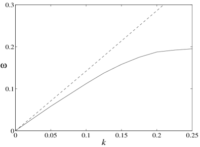
Figure 3: Phonon spectrum of a boson-fermion mixture. The Fermi gas is in a superfluid state. $a_{BF}=0$ for the dashed line, and $a_{BF}=0.1$ for the solid line. Other parameters are $a_{B}=0.04$, $n_{B}=1$ and $\Delta=0.1$. Same units as in Fig. 1.

Due to the form of ${\rm Re}[\tilde{\ell}_{k}(\omega)]$, the dispersion relation, $\omega(k)$, in the stable regime must be evaluated numerically. Fig. 3 shows $\omega(k)$ for the BCS state of the Fermi gas. In contrast to the normal state for the fermions, the BCS state results in an $\omega(k)$ that is reduced below that of the Bogoliubov spectrum of a pure condensate. Again, this is a result of the stability criterion (42), imposed on the energy of the excitation of the condensate. For the BCS state in the stable regime determined by (42), the density-density response function $\tilde{\ell}_{k}(\omega)$ is always negative. From Eq. (30), it follows that $\omega(k)$ is reduced in this case.

It is worth pointing out that when $\Delta\ll E_{F}$ (which is usually the case), one can show that $\tilde{\ell}_{k}(\omega)$ in the $k\rightarrow 0$ and $\omega=0$ static limit yields $\tilde{\ell}_{k}(0)\approx-8\pi m_{F}k_{F}/\hbar$, which agrees with the analytic result for the normal state of the Fermi gas [see Eq. (27)]. This indicates that the mechanical stability of the Bose-Fermi mixture does not depend on the state of the Fermi gas.

IV Conclusions

In this paper, by extending the standard Bogoliubov linearization procedure, we have analyzed the excitations of a weakly interacting Bose-Einstein condensate coupled to a degenerate Fermi gas at zero temperature. We derived general expressions for the excitations of the condensate in the presence of a Fermi gas that are valid for abitrary spatial geometries. When we specialized our results to the case of a spatially homogenous system, it was found that the quasiparticle spectrum for the condensate exhibits a dynamical instability due to the coupling between the Bose and Fermi gases. The instability corresponds to the resonant exchange of energy and momentum between the bosonic quasiparticle and pairs of quasiparticle excitations in the Fermi gas. In the stable regime, quantum fluctuations in the density of the Fermi gas modify the quasiparticle spectrum of the BEC. In the long wavelength limit, the speed of sound in the BEC is increased (decreased) when the Fermi gas is in the normal (superfluid) state as compared to the Bogoliubov speed of sound for a pure weakly interacting condensate. This difference arises from the different stability criteria [see Eqs. (29) and (42)] which are determined by the nature of the resonant coupling between the bosons and fermions in the mixture.

This paper lays the groundwork for the study of nonlinear wave-mixing between degenerate beams of bosons and fermions. Future work will extend the results obtained here for the equilibrium state of coupled Bose-Fermi gases to the nonequilibrium mixing of bosonic and fermionic matter waves. In contrast to the equilibrium case, where the instability signals the existence of a new ground state of the system, the existence of an instability in the nonequilibrium wave-mixing indicates exponential growth in one of the matter wave modes.

In the current work, we have focused on the quasiparticle excitation spectrum of the bosons in the mixture. Future work should include the study of the induced fermion-fermion coupling due to their interaction with bosons. This will shed light on the long-sought goal of inducing Cooper pairing of fermions using bosonic atoms viverit ; bijlsma .

V Appendix: Ground State with Correlated Bose-Fermi Densities

In this appendix we examine the ground state energy of a BEC collisionally coupled to a normal Fermi gas in a box of volume $V$. We show that a variational ground state wave function with a finite probability amplitude for excitations with opposite momentum in the BEC and the Fermi gas can result in an energy that is lower than that of the ground state used in Section II. The variational wave function we propose in this appendix is not necessarily the true ground state of the system, but instead provides an indication of the possible form of the ground state that the system evolves to in the presence of a dynamical instability.

The Hamiltonian, $\hat{H}^{\prime}$ for the Bose-Fermi mixture written in a plane wave basis has the form (note that in this appendix we do not use the grand canonical Hamiltonian),

$$\hat{H}^{\prime}=\hat{H}_{T}+\hat{H}_{BB}+\hat{H}_{BF},$$ (43)

where

$$\hat{H}_{T} = \sum_{{\bf k}}\left(\frac{\hbar^{2}k^{2}}{2m_{B}}\eta^{\dagger}_{{\bf k}}\eta_{{\bf k}}+\sum_{\sigma}\frac{\hbar^{2}k^{2}}{2m_{F}}a^{\dagger}_{{\bf k}\sigma}a_{{\bf k}\sigma}\right),$$

$$\hat{H}_{BB} = \frac{g_{B}}{2V}\sum_{{\bf k,k^{\prime},q}}\eta^{\dagger}_{{\bf k+q}}\eta^{\dagger}_{{\bf k^{\prime}-q}}\eta_{{\bf k^{\prime}}}\eta_{{\bf k}},$$

$$\hat{H}_{BF} = \frac{g_{BF}}{V}\sum_{\bf q}\zeta_{\bf q}\rho^{\dagger}_{{\bf q}}.$$

$\hat{H}_{T}$ represents the kinetic energy for the Bose and Fermi gases while $\hat{H}_{BB}$ is the collisional interaction between bosons. The boson-fermion interaction, $\hat{H}_{BF}$, has been expressed in terms of the operators for the ${\bf q}^{th}$ Fourier component of the fermion density,

$$\rho_{\bf q}=\sum_{{\bf k^{\prime}}\sigma}a^{\dagger}_{{\bf k^{\prime}+q}\sigma}a_{{\bf k^{\prime}}\sigma}$$ (44)

and the boson density,

$$\zeta_{\bf q}=\sum_{{\bf k^{\prime}}}\eta^{\dagger}_{{\bf k^{\prime}+q}}\eta_{{\bf k^{\prime}}}.$$ (45)

Note that $\rho_{-{\bf q}}=\rho^{\dagger}_{\bf q}$ and similarly, $\zeta_{-{\bf q}}=\zeta^{\dagger}_{{\bf q}}$. In contrast to Sections II and III, where the ${\bf k}=0$ condensate mode for the bosons was treated as a $c$-number, we now retain the operator dependence for the ${\bf k}=0$ mode, $\eta_{0}$, in the Hamiltonian. As in Sec. II, we neglect the direct fermion-fermion interaction.

In Sec. II, the equations of motion for the density fluctuations were linearized around the $T=0$ ground state for the non-interacting Bose and Fermi gases, $|\Psi_{N}\rangle$, which was implicitly assumed to remain a stable ground state for the interacting Bose-Fermi system. However, the existence of the dynamical instability indicates that $|\Psi_{N}\rangle$ is actually not stable and that there exists a ground state with a lower energy than $|\Psi_{N}\rangle$. The expectation value of the Hamiltonian with respect to $|\Psi_{N}\rangle$, $E_{N}=\langle\Psi_{N}|\hat{H}^{\prime}|\Psi_{N}\rangle$, is easily found to be,

$$E_{N}=2\sum_{k\leq k_{F}}\frac{\hbar^{2}k^{2}}{2m_{F}}+\frac{g_{B}}{V}\left(N_{B}^{2}-N_{B}\right)+\frac{2g_{BF}}{V}N_{B}N_{F}.$$ (46)

$|\Psi_{N}\rangle$ is equivalent to the ground state used in previous investigations of Bose-Fermi mixtures, in the sense that $|\Psi_{N}\rangle$ does not include any quantum correlations between the bosons and fermions, i.e. $|\Psi_{N}\rangle$ factorizes in to the product of the wave functions for the condensate and the ideal Fermi gas.

Any excitation with finite momentum in the two gases will increase the total kinetic energy, $\hat{H}_{T}$, but may result in a decrease in the interaction energy between the bosons and fermions. For example, consider the wave function,

$$|\Psi_{D}\rangle = \left(u_{\bf q}+v_{\bf q}\kappa^{-1}_{\bf q}\eta^{\dagger}_{\bf q}\eta_{0}\rho^{\dagger}_{{\bf q}}/\sqrt{N_{B}}\right)|\Psi_{N}\rangle$$

$$= \left(u_{\bf q}+v_{\bf q}\kappa^{-1}_{\bf q}\zeta_{\bf q}\rho_{-{\bf q}}/\sqrt{N_{B}}\right)|\Psi_{N}\rangle,$$

where $|u_{\bf q}|^{2}+|v_{\bf q}|^{2}=1$ and

$$\kappa_{\bf q}^{2}=\langle\Psi_{N}|\rho_{\bf q}\rho^{\dagger}_{\bf q}|\Psi_{N}\rangle=2\sum_{\bf k}\Theta(k_{F}-k)\Theta(|{\bf k-q}|-k_{F}).$$

The action of $\zeta_{\bf q}\rho_{-{\bf q}}$ on $|\Psi_{N}\rangle$ is to create a state with a density fluctuation of momentum $\hbar{\bf q}$ in the BEC along with a density fluctuation of momentum $-\hbar{\bf q}$ in the Fermi gas. It is easy to show that, just like $|\Psi_{N}\rangle$, $|\Psi_{D}\rangle$ corresponds to a spatially uniform state with densities $N_{B}/V$ and $2N_{F}/V$ for the Bose and Fermi gases, respectively. The difference between $|\Psi_{D}\rangle$ and $|\Psi_{N}\rangle$ is made manifest in the correlation between the boson and fermion densities,

$$\langle\Psi_{N}|\hat{\psi}_{B}^{\dagger}\hat{\psi}_{B}({\bf r})\sum_{\sigma}\hat{\psi}_{\sigma}^{\dagger}\hat{\psi}_{\sigma}({\bf r^{\prime}})|\Psi_{N}\rangle=\frac{N_{B}}{V}\frac{2N_{F}}{V},$$ (47)

$$\langle\Psi_{D}|\hat{\psi}_{B}^{\dagger}\hat{\psi}_{B}({\bf r})\sum_{\sigma}\hat{\psi}_{\sigma}^{\dagger}\hat{\psi}_{\sigma}({\bf r^{\prime}})|\Psi_{D}\rangle=\frac{N_{B}}{V}\frac{2N_{F}}{V}$$

$$+\frac{2\sqrt{N_{B}}\kappa_{\bf q}}{V^{2}}|u_{\bf q}||v_{\bf q}|\cos[{\bf q}\cdot({\bf r}-{\bf r^{\prime}})+\gamma],$$ (48)

where $\gamma=\arg(u^{*}_{\bf q}v_{\bf q})$ is the relative phase between $u_{\bf q}$ and $v_{\bf q}$. The density-density correlation for $|\Psi_{D}\rangle$ depends on the quantum coherences, $u_{\bf q}^{*}v_{\bf q}$, and can be made larger or smaller than (47) by varying $\gamma$. This can be used to lower the boson-fermion interaction energy since it is proportional to the spatially integrated density-density correlation between the two gases for ${\bf r}={\bf r^{\prime}}$.

The difference in the energy of the two states is

$$\Delta E = \langle\Psi_{D}|\hat{H}^{\prime}|\Psi_{D}\rangle-E_{N}$$

$$= E_{1}(q)v_{\bf q}^{2}+\frac{1}{2}E_{2}(q)\left(v_{\bf q}u^{*}_{\bf q}+v^{*}_{\bf q}u_{\bf q}\right).$$

$E_{1}(q)$ represents the increase in the kinetic energy and the mean field energy of the condensate,

$$E_{1}(q)=\frac{\hbar^{2}q^{2}}{2m_{B}}+2\kappa_{\bf q}^{-2}\sum_{k\leq k_{F}}^{|{\bf k-q}|>k_{F}}\left(\frac{\hbar^{2}q^{2}}{2m_{F}}-\frac{\hbar^{2}{\bf k\cdot q}}{m_{F}}\right)+2g_{B}\frac{N_{B}}{V},$$

while $E_{2}(q)$ is due to the boson-fermion interaction,

$$E_{2}(q)=2g_{BF}\sqrt{N_{B}}\kappa_{\bf q}/V.$$

Now let $v_{\bf q}=\sin\phi_{\bf q}$ and $u_{\bf q}=\pm\cos\phi_{\bf q}$ for $0\leq\phi_{\bf q}\leq\pi/2$. For $u_{\bf q}$, we use the upper sign for $g_{BF}<0$ and the lower sign for $g_{BF}>0$. By minimizing $\Delta E$ with respect to $\phi_{\bf q}$ one finds that the minimum value of the energy difference is

$$\Delta E_{min}=\frac{1}{2}\left[E_{1}(q)-\sqrt{E_{1}(q)^{2}+E_{2}(q)^{2}}\right],$$

which occurs when $\tan 2\phi_{\bf q}=|E_{2}(q)|/E_{1}(q)$. Note that $\Delta E_{min}<0$ for all values of ${\bf q}$, which indicates that quantum correlations between the densities of the two gases can lower the energy. Consequently, $|\Psi_{N}\rangle$ is not the true ground state of the Bose-Fermi mixture. To find the true ground state, $|\Psi_{D}\rangle$ would have to be extended to treat density fluctuations in all modes. This is a non-trivial task that will be the subject of future work.

We want to stress here that even though $|\Psi_{N}\rangle$ is not the lowest energy state, this does not necessarily mean that it is dynamically unstable. The relationship between the states $|\Psi_{D}\rangle$, $|\Psi_{N}\rangle$ and the dynamical stability condition, ${\rm Im}[\ell_{k}(\omega)]=0$, can be understood in the following manner. Suppose we start with the BEC and Fermi gas in separate unconnected boxes so that the quantum states for the Bose-Fermi system is factorizable into the product of the BEC state and the state of an ideal Fermi gas at $T=0$, namely $|\Psi_{N}\rangle$. If we then bring the two gases together in the same box so that they can interact, then $|\Psi_{N}\rangle$ will evolve into an entangled state with a form similar to $|\Psi_{D}\rangle$ provided that ${\rm Im}[\ell_{q}(\omega(q))]\neq 0$, where $\hbar\omega(q)$ is the energy of the density fluctuation in the BEC. This is because (a) correlations between the density fluctuations only develop if there is a coupling between the fluctuations in the two gases; and (b) since ${\rm Im}[\ell_{q}(\omega(q))]$ is proportional to the dynamic structure factor for the Fermi gas, it measures the strength of the resonant coupling between the two gases. If ${\rm Im}[\ell_{q}(\omega(q))]=0$, the density fluctuations in the two gases with momentum $\pm\hbar{\bf q}$ are uncoupled and there is no way to generate any quantum correlations between the two gases, thereby lowering the energy of the system.

This argument can be made quantitative if we evaluate the state of the Bose-Fermi system to first order in pertubation theory. If we work in the interaction representation where

$$\hat{H}_{BF}(t)=e^{i(\hat{H}_{T}+\hat{H}_{BB})t/\hbar}\hat{H}_{BF}e^{-i(\hat{H}_{T}+\hat{H}_{BB})t/\hbar},$$

then the state of the system at time $t$ starting from the ground state of the uncoupled system is, to first order in $g_{BF}$,

$$|\Psi(t)\rangle=\left(1-i\hbar^{-1}\int_{-\infty}^{t}dt^{\prime}\hat{H}_{BF}(t^{\prime})\right)|\Psi_{N}\rangle.$$

By letting $t\rightarrow\infty$ we obtain,

$$|\Psi(\infty)\rangle=\left(1-2i\pi g_{BF}\hbar^{-1}\sum_{\bf q}\eta^{\dagger}_{\bf q}\eta_{0}\left[\frac{1}{V}\sum_{{\bf k}\sigma}a^{\dagger}_{{\bf k-q}\sigma}a_{{\bf k}\sigma}\delta\left(\omega(q)-\hbar({\bf k-q})^{2}/2m_{F}+\hbar{\bf k}^{2}/2m_{F}\right)\right]\right)|\Psi_{N}\rangle,$$ (49)

which has a form similar to that of $|\Psi_{D}\rangle$ generalized to include all modes for the coupled density fluctuations. The delta function implies that correlations are dynamically generated between $\zeta_{{\bf q}}$ and those components of $\rho_{\bf q}$ that conserve energy in the $t\rightarrow\infty$ limit. Note that $\hbar\omega(q)$ in Eq. (49) is equal to the energy of a Bogoliubov quasipaticle in the uncoupled BEC since dispersive effects due to the Bose-Fermi coupling are higher order in $g_{BF}$. From $|\Psi(\infty)\rangle$, one sees that the interaction between the bosons and fermions will naturally lead to an entangled state provided the term in brackets is nonzero. It is easy to see from Eq. (25) that

$$\left[\sum_{{\bf k}\sigma}a^{\dagger}_{{\bf k-q}\sigma}a_{{\bf k}\sigma}\delta\left(\omega(q)-\frac{\hbar({\bf k-q})^{2}}{2m_{F}}+\frac{\hbar{\bf k}^{2}}{2m_{F}}\right)\right]|\Psi_{N}\rangle=0,$$

unless ${\rm Im}[\ell_{-q}(\omega(-q))]\neq 0$. Note that for an isotropic system, ${\rm Im}[\ell_{-q}(\omega(-q))]={\rm Im}[\ell_{q}(\omega(q))]$.

To summarize, we have shown that the existence of a dynamical instability indicates that entanglement between the Bose and Fermi systems can be dynamically generated by $\hat{H}_{BF}$ starting from the factorizable state $|\Psi_{N}\rangle$. In this case, a variational wave function such as $|\Psi_{D}\rangle$ that involves an entanglement between density fluctuations in the two gases with opposite momenta can have lower energy than $|\Psi_{N}\rangle$.

References

(1) M. H. Anderson et al., Science 269, 198 (1995);
K. B. Davis et al., Phys. Rev. Lett. 75, 3969 (1995);
C. C. Bradley et al., Phys. Rev. Lett. 75, 1687
(1995).
(2) B. DeMarco et al., Phys. Rev. Lett. 86, 5409 (2001).
(3) M. J. Holland, B. DeMarco, and D. S. Jin, Phys.
Rev. A 61, 053610 (2000).
(4) H. T. C. Stoof et al., Phys. Rev. Lett 76, 10
(1996); M. Houbiers et al., Phys. Rev. A 56, 4864
(1997).
(5) G. Bruun, Y. Castin, R. Dum, and K. Burnett,
Eur. Phys. J. D 7, 433(1999).
(6) J. L. Bohn, Phys. Rev. A 61, 053409 (2000);
T. Loftus et al., e-print cond-mat/0111571.
(7) M. Holland et al., Phys. Rev. Lett. 87,
120406 (2001).
(8) M. Mackie et al., Opt. Express 8, 118
(2000); M. Mackie et al., e-print physics/0104043.
(9) A. G. Truscott et al., Science 291, 2570
(2001); F. Schreck et al., Phys. Rev. Lett. 87, 080403
(2001).
(10) S. R. Granade et al., cond-mat/0111344.
(11) B. DeMarco and D. S. Jin, Science 285, 1703
(1999).
(12) Eddy Timmermans, Phys. Rev. Lett. 87, 240403
(2001).
(13) J. Goldwin, S. B. Papp, B. Demarco, and D. S. Jin,
e-print cond-mat/0108287.
(14) K. Molmer, Phys. Rev. Lett. 80, 1804
(1998).
(15) L. Viverit, C. J. Pethick, and H. Smith, Phys.
Rev. A 61, 053605(2000).
(16) R. Roth and H. Feldmeir, cond-mat/0108524.
(17) X. X. Yi and C. P. Sun, Phys. Rev. A 64,
043608(2001).
(18) S. K. Yip, Phys. Rev. A 64, 023609(2001).
(19) M. J. Bijlsma, B. A. Heringa, and H. T. C.
Stoof, Phys. Rev. A 61, 053601 (2000).
(20) P. Capuzzi and E. S. Hernandez, Phys. Rev. A 64, 043607(2001).
(21) A. Minguzzi and M. P. Tosi, Phys. Lett. A 268, 142 (2000).
(22) M. A. Baronov and D. S. Petrov, Phys. Rev. A
62, R041601 (2000).
(23) A. Minguzzi, G. Ferrari, and Y. Castin,
cond-mat/0103591.
(24) G. M. Bruun and B. R. Mottelson,
cond-mat/0107628.
(25) G. M. Bruun and C. W. Clark, J. Phys. B 33, 3953 (2000);
M. A. Baranov, JETP Lett. 70, 396 (1999).
(26) N. N. Bogoliubov, J. Phys. USSR 11, 23
(1947).
(27) H. Pu et al., e-print cond-mat/0104279.
(28) M. G. Moore and P. Meystre, Phys. Rev. Lett. 86, 4199 (2001).
(29) S. Inouye et al., Science 285, 571
(1999).
(30) P. Nozieres and D. Pines, The Theory of Quantum
Liquids Vol. I (Perseus Books, Reading, MA, 1999).
(31) A. L. Fetter and J. D. Walecka, Quantum Theory of
Many-Particle Systems (McGraw Hill, New York 1971).
(32) P. Meystre and M. Sargent III, Elements of
Quantum Optics 3rd. Ed. (Springer, New York, 1999).
(33) P. G. DeGennes, Superconductivity of
Metals and Alloys (W. A. Benjamin, New York, 1966).
(34) N. N. Bogoliubov, Nuovo Cimento 7, 794
(1958); Sov. Phys. JETP 7, 41 (1958).
(35) M. Tinkham, Introduction to
Superconductivity 2nd ed. (McGraw-Hill, New York, 1996).