Physics of Psychophysics: Stevens and Weber-Fechner laws are transfer functions of excitable media

Abstract

Sensory arrays made of coupled excitable elements can improve both their input sensitivity and dynamic range due to collective non-linear wave properties. This mechanism is studied in a neural network of electrically coupled (e.g. via gap junctions) elements subject to a Poisson signal process. The network response interpolates between a Weber-Fechner logarithmic law and a Stevens power law depending on the relative refractory period of the cell. Therefore, these non-linear transformations of the input level could be performed in the sensory periphery simply due to a basic property: the transfer function of excitable media.

A very common trade-off problem found in the biology of sensory mechanisms (and sensor devices in general) is the competition between two desirable goals: high sensitivity (the system ideally should be able to detect even single signal events) and large dynamic range (the system should not saturate over various orders of magnitude of input intensity). In physiology, for example, broad dynamic ranges are related to well known psychophysical laws Stevens ; BBS : the response $R$ of the sensory system may be proportional not to the input level $I$ but to its logarithm, $R\propto\ln I$ (Weber-Fechner Law) or to a power of it, $R\propto I^{\alpha},\>(\alpha<1)$ (Stevens Law).

Most of the attempts to explain these psychophysics laws consist basically in top-down approaches trying to show that they could be derived from some optimization criterium for information processing BBS ; Chater . In this work we use a botton-up, statistical mechanics approach, showing how these laws emerge from a microscopic level. Indeed, they are generic transfer functions of excitable media subjected to external (Poisson) input. Of course, this does not explain “why” these laws have been adopted by Biology (some optimization criterium may be relevant here), but explains why Biology uses excitable media to implement them.

Receptor cells of sensory systems are electrically coupled via gap junctions Dorries ; ZM . However, the functional roles of this electrical coupling are largely unknown. Here we report a simple mechanism that could increase at the same time the sensitivity and the dynamic range of a sensory epithelium by using only this electrical coupling. The resulting effect is to transform the individual linear-saturating curves of individual cells into a collective Weber-Fechner like logarithmic response curve with high sensitivity to single events and large dynamic range. We also observe a change to power law behavior (Stevens Law) if relative refractory periods are introduced in the model.

Although the phenomenon discusssed in this work could be illustrated at different modeling levels Kinouchi , we have chosen here to work with the simplest elements: cellular automata (CA). The simplicity of the model supports our case that the mechanisms underlying the described phenomena are very general. To confirm this picture, we also present preliminary results for neurons modeled by the Hodgkin-Huxley equations.

The $n$-state CA model is an excitable element containing two ingredients: 1) a cell spikes only if stimulated while in its resting state and 2) after a spike, a refractory period takes place, during which no further spikes occur, until the cell returns to its resting state. Denoting the state of the $i$-th cell at time $t$ by $x_{i}(t)\in\{0,1,\ldots,n-1\}$, the dynamics of the proposed CA can be simply described by the following rules:

1. If $x_{i}(t)=0$, then $x_{i}(t+1)=h_{i}(t)$, where $h_{i}\in\{0,1\}$.

2. If $x_{i}(t)\neq 0$, then $x_{i}(t+1)=[x_{i}(t)+1]\mod n$.

Interpretation of the above rules is straightforward: a cell only responds to stimuli in its resting state ($x_{i}=0$). If there is no stimulus ($h_{i}=0$), it remains unchanged. In case of stimulus ($h_{i}=1$), it responds by spiking ($x_{i}=1$) and then remaining insensitive to further stimuli during $n-2$ time steps ($x_{i}\in\{2,\ldots,n-1\}$).

In what follows, we assume that the external input signal $I_{i}(t)$ arriving on cell $i$ at time $t$ is modeled by a Poisson process of supra-threshold events of stereotyped unit amplitude: $I_{i}(t)=\sum_{n}\delta\left(t,t^{(i)}_{n}\right)$ where $\delta(a,b)$ is the Kronecker delta and the time intervals $t^{(i)}_{n+1}-t^{(i)}_{n}$ are distributed exponentially with average (input rate) $r$, measured in events per second. For uncoupled cells, we have then simply $h_{i}(t)=\delta\left(I_{i}(t),1\right)$.

In order to visualize the effect of the refractory period, we mimick the behavior of the spike of a neuron by mapping the automaton state into an action potential wave form

$$V(x_{i}) = V_{0}\left\{\frac{}{}\delta(x_{i},1)-\left[1-\delta(x_{i},0)\right]\left[1-\delta(x_{i},1)\right]\right.$$ (1)

$$\left.\times k\left(1-\frac{(x_{i}-2)}{n-2}\right)\right\}\;.$$

Notice that $V$ plays no role whatsoever in the dynamics. Fig. 1(a) shows the behavior of $V(x_{i}(t))$ for an uncoupled 5-state automaton. We observe that stimuli that fall within the refractory period go undetected, and in the absence of stimuli the automaton eventually returns to and stays at its quiescent state $x_{i}=0$. Since a typical spike lasts the order of 1 ms, this provides a natural time scale of 1 ms per time step, which will be used throughout this paper.

Figure 1: Time evolution for $n=5$: (a) $V(x(t))$ for a single uncoupled cell (solid lines) and stimuli $h(t)$ (bars) at $r=100$ events/sec with $V_{0}=5$ and $k=0.3$; (b) system with $L=50$ coupled cells at $r=10$ events/sec: $x_{i}=1$ (filled circles), $2\leq x_{i}\leq n-1$ (open circles) and $x_{i}=0$ (white background). Arrows indicate events to be considered in more detail subsequently.

Response of uncoupled receptor cells is shown in Fig. 2 (thick lines on top panels). We draw input signals at rate $r$ per cell and measure the average firing rate $f$ (spikes per second per cell) of the $n$-state automata over a sufficiently long time. In the low rate regime the activity of the uncoupled cells is proportional to the signal rate. If the rate increases, there is a deviation from the linear behavior due to the cell’s refractory time $\Delta_{n}\equiv n\times 10^{-3}$ seconds. The single-cell response $f$ is extremely well fitted by a linear-saturating curve $f_{n}$ [Fig 2(a) and (b)]:

$$f_{n}(r)=r/(1+r\Delta_{n})\>,$$ (2)

which can be deduced from the fact that the firing rate is proportional to the rate discounting the refractory intervals, $f_{n}=r(1-f_{n}\Delta_{n})$. The same result can be obtained by a stationary mean field solution of the uncoupled cells.

How to improve the sensitivity for very low rates? If we consider the response $R$ (spikes per second) of the total pool of $L$ independent cells, we have $R=Lf\approx Lr$, so increasing $L$ increases the total sensitivity of the epithelium. Although certainly useful, this scaling is trivial since the efficiency of each cell remains the same.

Coupled excitable cells (say, via gap junctions) are an example of excitable media that supports the propagation of nonlinear waves Murray . Here we show that the formation and annihilation of these waves enhance the sensitivity and, at the same time, extends the dynamic range of a sensory epithelium. We couple $L$ cellular automata in a chain by defining the local input as

$$h_{i}(t)=1-\left[1-\delta(I_{i}(t),1)\right]\prod_{j=\pm 1}\left[1-\delta(x_{i+j}(t),1)\right]\;,$$ (3)

i.e. $h_{i}(t)$ will be nonzero whenever either of $i$’s neighbors are spiking and/or the external input is nonzero. This kind of coupling models electric gap junctions instead of chemical synapses because it is fast and bidirectional.

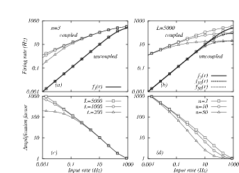
Figure 2: Firing rates $f$ and $F$ (top) and amplification factor $A$ (bottom) vs. input rate $r$ for $n=3$ and varying $L$ [(a) and (c)] and for $L=5000$ and varying $n$ [(b) and (d)]. Thick lines (top panels) show $f_{n}(r)$ as in Eq. 2.

A sample of the resulting chain dynamics is shown in Fig. 1(b). Due to coupling, single input events create waves that propagate along the chain, leaving behind a trail of refractoriness (of width $n-1$) which prevents new spikes from reappearing immediately. More importantly, refractoriness is responsible for wave annihilation: when two wave fronts meet at site $i$ they get trapped because the neighboring sites have just been visited and are still in their refractory period. This is a well known phenomenon in excitable media Murray and occurs in the CA model $\forall n\geq 3$. Notice that the overall shape of two consecutive wave-fronts are correlated (see Fig. 1), denoting some kind of memory effect, a phenomenon observed previously by Chialvo et al. Chialvo and Lewis and Rinzel Lewis .

Due to a chain-reaction mechanism, the spike of a single receptor cell is able to excite all the other cells. The sensitivity per neuron has thus increased by a factor of $L$. This can be clearly seen in Fig. 2, which shows the average firing rate per cell $F$ in the coupled system (top panels), as well as the amplification factor $A\equiv F/f$ (bottom panels). This is a somewhat expected effect of the coupling: neuron $j$ is excited by signal events that arrive not only at neuron $j$ but elsewhere in the network.

More surprising is the fact that the dynamic range (the interval of rates where the neuron produces appreciable but still non-saturating response) also increases dramatically. This occurs due to a second effect, which we call the self-limited amplification effect. Remember that a single spike of some neuron produces a total of $L$ neuronal responses. This is valid for small rates, where inputs are isolated in time from each other. However, for higher signal rates, a new event occurs at neuron $k$ before the wave produced by neuron $j$ has disappeared. If the initiation site $k$ is inside the fronts of the previous wave [e.g. the events signaled by arrows in Fig. 1(b)], then two events produce $2L$ responses as before. But if $k$ is situated outside the fronts of the $j$-initiated wave [as in the first input events shown in Fig. 1(b)], one of its fronts will run toward the $j$-wave and both fronts will annihilate.

Thus, two events in the array have produced only $L$ excitations (that is, an average of $L/2$ per input event). So, in this case, the efficiency for two consecutive events (within a window defined by the wave velocity and the size $L$ of the array) has been decreased by half. If more events (say, $m$) arrive during a time window, many fronts coexist but the average amplification of these $m$ events (how many neurons each event excites) is only of order $L/m$.

Therefore, although the amplification for small rates is very high, saturation is avoided due to the fact that the amplification factor decreases with the rate in a self-organized non-linear way. The amplification factor $A$ shown in Figs. 2(c) and 2(d) decreases in a sigmoidal way from $A={\cal O}(L)$ for very small rates (since a single event produces a global wave) to $A=1$ for large rates, where each cell responds as if isolated since waves have no time to be created or propagate.

The role of the system size $L$ for low input rates becomes clear in Fig. 2(c): the larger the system, the lower the rate $r$ has to be in order for the amplification factor to saturate at ${\cal O}(L)$. In other words, we can think of a decreasing crossover value $r_{1}(L)$ such that the response is well approximated by $F(r)=Lf(r)\approx Lr$ for $r\ll r_{1}(L)$. In this linear regime consecutive events essentially do not interact. Larger system sizes increase not only the overall rate of wave creation ($\sim 1-(1-r)^{L}$) but also the time it takes for a wave to reach the borders and disappear. In the opposite limit of large input rates, the behavior of the response is controlled by the absolute refractory period $\Delta$, as shown in Fig. 2: $F$ and $f$ saturate at $r_{2}\equiv 1/\Delta$ for $f\gtrsim r_{2}$, independently of the system size.

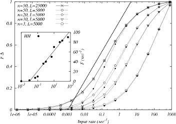
Figure 3: $F\times\Delta$ vs. input rate $r$ for $L=5000$ (open symbols) and $L=200$ (filled symbols) for different values of $n$. A $L=25000$ curve for $n=50$ (crosses) shows no difference to the $L=5000$ case. Straight lines are intended as a guide to the eye. Inset: $F(r)$ for the Hodgkin-Huxley system.

So what happens for intermediate input rates, i.e. $r_{1}\ll r\lesssim r_{2}$? The answer is a slow, Weber-Fechner-like increase in the response $F$, as can be seen in Fig. 3. The logarithmic dependence on $r$ is a good fit of the curves for about three decades.

Motivated by results obtained with more realistic elements Kinouchi we introduced a relative refractory period in our CA model. We first define a time window $M$ after a spike during which no further spikes can occur (absolute refractory period). In the following $n-M-2$ steps (relative refractory period), a single input does not produce a spike but two or more inputs can elicit a cell spike if they arrive within a temporal summation window $\tau$ (details of this model will be described in a forthcoming full paper). This ingredient produced the appearance of a power law $F(r)$ curve (Stevens Law Stevens ; BBS ), as shown in Fig. 4. Notice that the exponent depends on the relative refractory period. The appearence of a power law transfer function is a robust effect also observed in coupled maps systems Kinouchi .

Figure 4: Neuronal “Stevens Law” $F\propto r^{\alpha}$ in automata which takes temporal summation effects into account (see text for details). Firing rate $F$ vs. input rate $r$ for a CA with $n$ states and an absolute refractory period of $M=3$ time steps. Filled circles: $n=15$, $\tau=10$, $\alpha=0.38$; open circles: $n=100$, $\tau=80$, $\alpha=0.44$.

We may confirm the generic character of the self-regulated amplification phenomenon by performing simulations using biophysically detailed cell models, for example a network of Hodgkin-Huxley (HH) elements with the standard set of parameters given in Genesis connected via gap junctions of $30M\Omega$. Preliminary results show that this system exbits the same qualitative behavior of the simple CA model (see inset of Fig. 3 and Fig. 5). More detailed results will be reported elsewhere.

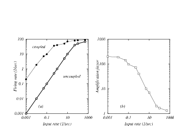
Figure 5: (a) Firing rate for coupled ($F$, filled circles) and uncoupled ($f$, open circles) systems and (b) amplification factor $A=F/f$ vs. input rate $r$ for Hodgkin-Hukley neurons for $L=200$.

Concerning the functional role of gap junctions for signal processing, it has been recognized that they provide faster communication between cells than chemical synapses and play a role in the synchronization of cell populations Traub . Here we are proposing another functional role for gap junctions: the enhancement of the dynamic range of neural networks.

There is considerable debate about what is the most appropriate functional law to describe psycophysical response: Weber-Fechner, Stevens or some interpolation between the two BBS . Our results suggest that properties of excitable media could be a bottom-up mechanism which can generate both laws, and a cross-over between them, depending on the presence of secondary factors like the relative refractory periods and temporal summation.

We can even make two more specific predictions which are easily testable experimentally: 1. The larger the relative refractory period (e.g., due to slower hyperpolarizing currents) of sensory epithelia neurons, the larger the exponent of Stevens Law; 2. For sufficiently low input rates, the sensory epithelium response will be always linear ($\alpha=1$).

This mechanism for amplified but self-limited response due to wave annihilation promotes signal compression, is a basic property of excitable media and is not restricted to one dimensional systems. We conjecture that the same mechanism could be implemented at different biological levels, from hippocampal networks (where axo-axonal gap junctions have been recently reported Traub and modeled Lewis by a CA similar to ours) to excitable dendritic trees in single neurons Chialvo ; Koch . This signal compression mechanism could also be implemented in artificial sensors based on excitable media.

Acknowledgments: Research supported by FAPESP, CNPq and FAPERJ. The authors thank Silvia M. Kuva for valuable suggestions and the referees for useful comments. OK thanks the hospitality of Prof. David Sherrington and the Theoretical Physics Department of Oxford University where these ideas have been first developed.

References

- (1) S. S. Stevens, Psychophysics: Introduction to its perceptual, neural and social prospects, ed. G. Stevens (Wiley, New York, 1975).
- (2) L. E. Krueger, Behav. Brain Sci. 12, 251 (1989).
- (3) N. Chater and G. D. A Brown, Cognition 69 B17-B24 (1999).
- (4) K. M. Dorries and J. S. Kauer, J. Neurophysiol. 83, 754 (2000).
- (5) D-Q. Zhang and D. G. McMahon, PNAS 97, 14754 (2000).
- (6) O. Kinouchi, to be published.
- (7) J. D. Murray, Mathematical Biology (Springer Verlag, Berlin, 1993).
- (8) D. R. Chialvo, G. A. Cecchi and M. O. Magnasco, Phys. Rev. E 61 5654 (2000).
- (9) T. J. Lewis and J. Rinzel, Network: Comput. Neural. Syst. 11, 299 (2000).
- (10) J. M. Bower and D. Beeman, The book of Genesis: exploring realistic neural models with the GEneral NEural SImulation System (Springer Verlag, New York, 1998).
- (11) R. D. Traub, D. Schmitz, J. G. R. Jefferys and A. Draguhn, Neuroscience 92, 407 (1999).
- (12) P. B. Detwiler, A. L. Hodgkin and P. A. McNaughton, J. Physiol. 300, 213 (1980).
- (13) C. Koch, Biophysics of Computation (Oxford University Press, Oxford, 1999).