Coupled Growing Networks

Abstract

We introduce and solve a model which considers two coupled networks growing simultaneously. The dynamics of the networks is governed by the new arrival of network elements (nodes) making preferential attachments to pre-existing nodes in both networks. The model segregates the links in the networks as intra-links, cross-links and mix-links. The corresponding degree distributions of these links are found to be power-laws with exponents having coupled parameters for intra- and cross-links. In the weak coupling case the model reduces to a simple citation network. As for the strong coupling, it mimics the mechanism of the web of human sexual contacts.

I Introduction

Today, with a vast amount of publications being produced in every discipline of scientific research, it can be rather overwhelming to select a good quality work; that is enriched with original ideas and relevant to scientific community. More often this type of publications are discovered through the citation mechanism. It is believed that an estimate measure for scientific credibility of a paper is the number of citations that it receives, though this should not be taken too literally since some publications may have gone unnoticed or have been forgotten about over time.

Knowledge of how many times their publications are cited can be seen as good feedback for the authors, which brings about an unspoken demand for the statistical analysis of citation data. One of the impressive empirical studies on citation distribution of scientific publications [1] showed that the distribution is a power-law form with exponent $\gamma\approx 3$. The power-law behaviour in this complex system is a consequence of highly cited papers being more likely to acquire further citations. This was identified as a preferential attachment process in [2].

The citation distribution of scientific publications is well studied and there exist a number of network models [3, 4, 5] to mimic its complex structure and empirical results [1, 6] to confirm predictions. However, they seem to concentrate on the total number of citations without giving information about the issuing publications. The scientific publications belonging to a particular research area do not restrict their references to that discipline only, they form bridges by comparing or confirming findings in other research fields. For instance most Small World Network Models [7, 8, 9] presented in statistical mechanics, reference a sociometry article [10] which presents the studies of Milgram on the small world problem. This is the type of process which we will investigate with a simple model that only considers two research areas and referencing within and across each other. The consideration of cross linking also makes the model applicable to the web of human sexual contacts [11, 12], where the interactions between males and females can be thought of as two coupled growing networks.

This paper is organized as follows: In the proceeding section the model is defined and analyzed with a rate equation approach [13, 14]. In the final section discussions and comparisons of findings with the existing data are presented.

II The model

One can visualize the proposed model with the aid of Fig. (1) that attempts to illustrate the growth mechanism. We build the model by the following considerations.

Initially, both networks $A$ and $B$ contains $m_{0}$ nodes with no cross-links between the nodes in the networks. At each time step two new nodes with no incoming links, one belonging to network $A$ and the other to $B$, are introduced simultaneously. The new node joining to $A$ with $m_{A}\leq m_{0}$ outgoing links, attaches $p_{AA}$ fraction of its links to pre-existing nodes in $A$ and $p_{AB}=1-p_{AA}$ fraction of them to pre-existing nodes in $B$. The similar process takes place when a new node joins to $B$, where the new node has $m_{B}\leq m_{0}$ outgoing links from which $p_{BB}$ of them goes to nodes in $B$ and the complementary $p_{BA}=1-p_{BB}$ goes to $A$. The attachments to nodes in either networks are preferential and the rate of acquiring a link depends on the number of connections and the initial attractiveness of the pre-existing nodes.

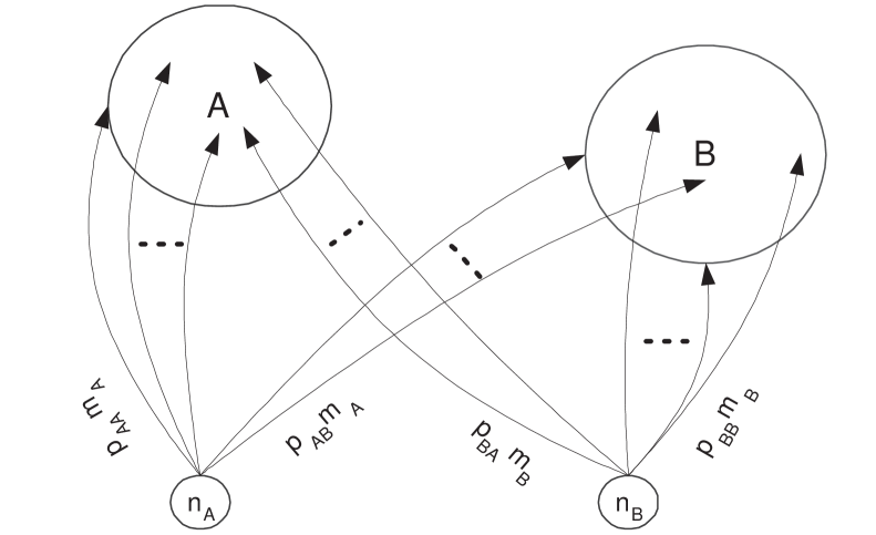
FIG. 1.: Schematic illustration of the growth processes of network $A$ and $B$. Each new node $n_{A}$ or $n_{B}$ is making a fractional cross linking to other network as well as intra links to their own .

We define $N_{A}(k_{A},t)$ as the average number of nodes with total $k_{A}$ number of connections that includes the incoming intra-links $k_{AA}$ and the incoming cross-links $k_{BA}$ in network $A$ at time $t$. Similarly, $N_{B}(k_{B},t)$ is the average number of nodes with $k_{B}=k_{BB}+k_{AB}$ connections at time $t$ in network $B$. Notice that the indices are discriminative and the order in which they are used is important, as they indicate the direction that the links are made. Further more we also define $N_{AA}(k_{AA},t)$ and $N_{BB}(k_{BB},t)$ the average number of nodes with $k_{AA}$ and $k_{BB}$ incoming intra-links to $A$ and $B$ respectively. Finally, we also have $N_{BA}(k_{BA},t)$ and $N_{AB}(k_{AB},t)$ to denote the average number of nodes in $A$ and $B$ with $k_{BA}$ and $k_{AB}$ incoming cross-links.

To keep this paper less cumbersome we will only analyse the time evolution of network $A$ and apply our results to network $B$. In addition to this, we only need to give the time evolution of $N_{A}(k_{AA},k_{BA},t)$, defined as the joint distribution of intra-links and cross-links. Using this distribution we can find all other distributions that are mentioned earlier. The time evolution of $N_{A}(k_{AA},k_{BA},t)$ can be described by a rate equation

$$\frac{dN_{A}(k_{AA},k_{BA},t)}{dt} = \frac{1}{M_{A}(t)}\{p_{AA}m_{A}[(k_{AA}-1+k_{BA}+a)N_{A}(k_{AA}-1,k_{BA},t)$$ (4)

$$-(k_{AA}+k_{BA}+a)N_{A}(k_{AA},k_{BA},t)]$$

$$+p_{BA}m_{B}[(k_{AA}+k_{BA}-1+a)N_{A}(k_{AA},k_{BA}-1,t)$$

$$-(k_{AA}+k_{BA}+a)N_{A}(k_{AA},k_{BA},t)]\}+\delta_{k_{AA}0}\delta_{k_{BA}0}.$$

The form of the Eq. (4) seems very similar to the one used in [15]. In that model the rate of creating links depends on the out-degree of the issuing nodes and the in-degree of the target nodes. Here we are concerned with two different types of in-degrees namely intra- and cross-links of the nodes.

On the right hand side of Eq. (4) the terms in first square brackets represent the increase in the number of nodes with $k_{A}$ links when a node with $k_{AA}-1$ intra-links acquires a new intra-link and if the node already has $k_{A}$ links this leads to reduction in the number. Similarly, for the second square brackets where the number of nodes with $k_{A}$ links changes due to the incoming cross-links. The final term accounts for the continuous addition of new nodes with no incoming links, each new node could be thought of as the new publication in a particular research discipline. The normalization factor $M_{A}(t)$ sum of all degrees is defined as

$$M_{A}(t)=\sum_{k_{A}=0}^{\infty}A_{k_{A}}N_{A}(k_{A},t).$$ (5)

We limit ourself to the case of preferential linear attachment rate[13]

$$A_{k_{A}}=a+k_{A},$$ (6)

shifted by $a>0$, the initial attractiveness [4] of nodes in $A$, which ensures that there is a nonzero probability of any node acquiring a link. The nature of $A_{k_{A}}$ lets one to obtain, as $t\to\infty$

$$M_{A}(t)=(a+<m_{A}>)t,$$ (7)

where $<m_{A}>=p_{AA}m_{A}+p_{BA}m_{B}$ is the average total in-degree in Network $A$. Eq. (7) implying that $M_{A}(t)$ is linear in time. Similarly, it is easy to show that $N_{A}(k_{AA},k_{BA},t)=n_{A}(k_{AA},k_{BA})t$ is also linear function of time. We use these relations in Eq. (4) to obtain the time independent recurrence relation

$$[a+<m_{A}>+<m_{A}>(k_{AA}+k_{BA}+a)]n_{A}(k_{AA},k_{BA})$$ (8)

$$=p_{AA}m_{A}(k_{AA}+k_{BA}+a-1)n_{A}(k_{AA}-1,k_{BA})$$ (9)

$$+p_{BA}m_{B}(k_{AA}+k_{BA}+a-1)n_{A}(k_{AA},k_{BA}-1)$$ (10)

$$+(a+<m_{A}>)\delta_{k_{AA}0}\delta_{k_{BA}0}.$$ (11)

The expression in Eq. (8) does not simplify however, it lets us to obtain the total in-degree distribution

$$N_{A}(k_{A},t)=\sum_{k_{AA}=0}^{k_{A}}N_{A}(k_{AA},k_{A}-k_{AA},t).$$ (12)

Writing $N_{A}(k_{A},t)=n_{A}(k_{A})t$ and since $k_{A}=k_{AA}+k_{BA}$ then $n_{A}(k_{A})$ satisfies

$$[a+<m_{A}>+<m_{A}>(k_{A}+a)]n_{A}(k_{A})=<m_{A}>(k_{A}+a-1)n_{A}(k_{A}-1)$$ (13)

$$+(a+<m_{A}>)\delta_{k_{A}0}.$$ (14)

Solving Eq. (13) for $k_{A}>0$ yields,

$$n_{A}(k_{A})=\frac{\Gamma(k_{A}+a)\Gamma(a+2+\frac{a}{<m_{A}>})}{\Gamma(k_{A}+a+2+\frac{a}{<m_{A}>})\Gamma(a)}n_{A}(0),$$ (15)

with

$$n_{A}(0)=\left(1+\frac{<m_{A}>a}{<m_{A}>+a}\right)^{-1}.$$ (16)

As $k_{A}\to\infty$ Eq. (15) gives the asymptotic behaviour of the total in-degree distribution in $A$

$$n_{A}(k_{A})\sim k_{A}^{-\gamma_{A}},$$ (17)

which is a power-law form with an exponent $\gamma_{A}=2+a/<m_{A}>$ that only depends on the average total in-degree and the initial attractiveness of the nodes. Similarly, we can write the total in-degree distribution in network $B$ for the asymptotic limit of $k_{B}$ as

$$n_{B}(k_{B})\sim k_{B}^{-\gamma_{B}}\quad\text{with}\quad\gamma_{B}=2+b/<m_{B}>.$$ (18)

Again, the exponent depends upon the initial attractiveness $b$ of nodes and the average total incoming links $<m_{B}>=p_{BB}m_{B}+p_{AB}m_{A}$.

We now move on to analyse $N_{AA}(k_{AA},t)$, the distribution of the average number of nodes with $k_{AA}$ intra-links in network $A$. In citation network one can think of these links being issued from the same subject class as the receiving nodes and in the case of human sexual contact network, they represent the homosexual interactions. Since

$$N_{AA}(k_{AA},t)=\sum_{k_{BA}=0}^{\infty}N_{A}(k_{AA},k_{BA},t),$$ (19)

which can also be written as $N_{AA}(k_{AA},t)=n_{AA}(k_{AA})t$, a linear function of time. Then summing Eq. (8) over all possible values of $k_{BA}$

$$n_{A}(k_{AA})=\sum_{k_{BA}=0}^{\infty}n_{A}(k_{AA},k_{BA}),$$ (20)

we get

$$[a+<m_{A}>+<m_{A}>(k_{AA}+a)]n_{AA}(k_{AA})+<m_{A}>\sum_{k_{BA}=0}^{\infty}k_{BA}n_{A}(k_{AA},k_{BA})$$ (21)

$$=p_{AA}m_{A}(k_{AA}+a-1)n_{AA}(k_{AA}-1)+p_{AA}m_{A}\sum_{k_{BA}=0}^{\infty}k_{BA}n_{A}(k_{AA}-1,k_{BA})$$ (22)

$$+p_{BA}m_{B}(k_{AA}+a)n_{AA}(k_{AA})+p_{BA}m_{B}\sum_{k_{BA}=0}^{\infty}(k_{BA}-1)n_{A}(k_{AA},k_{BA}-1)$$ (23)

$$+(a+<m_{A}>)\delta_{k_{AA}0}.$$ (24)

For large $k_{AA}$ Eq. (21) reduces to

$$[a+<m_{A}>+p_{AA}m_{A}(k_{AA}+a)]n_{AA}(k_{AA})=$$ (25)

$$p_{AA}m_{A}(k_{AA}+a-1)n_{AA}(k_{AA}-1)+(a+<m_{A}>)\delta_{k_{AA}0}.$$ (26)

Iterating former relation for $k_{AA}>0$ yields

$$n_{AA}(k_{AA}) = \frac{\Gamma(k_{AA}+a)\Gamma(a+2+\frac{p_{BA}m_{B}+a}{p_{AA}m_{A}})}{\Gamma(k_{AA}+a+2+\frac{p_{BA}m_{B}+a}{p_{AA}m_{A}})\Gamma(a)}n_{AA}(0),$$ (27)

where

$$n_{AA}(0)=(1+\frac{p_{AA}m_{A}a}{a+<m_{A}>})^{-1}.$$ (28)

In the asymptotic limit as $k_{AA}\to\infty$ Eq. (27) has a power-law form

$$n_{AA}(k_{AA})\sim k_{AA}^{-\gamma_{AA}},\quad\text{with exponent}\quad\gamma_{AA}=2+\frac{p_{BA}m_{B}+a}{p_{AA}m_{A}}$$ (29)

that depends upon both $p_{AA}$ and the coupling parameter $p_{BA}$.

Similarly, the time independent recurrence relation for $N_{BB}(k_{BB},t)$ has the same form as Eq. (21) with the only difference being the parameters. Therefore we will simply give the power-law distribution

$$n_{BB}(k_{BB})\sim k_{BB}^{-\gamma_{BB}}\quad\text{with}\quad\gamma_{BB}=2+\frac{p_{AB}m_{A}+b}{p_{BB}m_{B}},$$ (30)

where the other coupling parameter $p_{AB}$ is revealed in the exponent.

Finally, the distribution of average number of nodes with incoming cross-links $N_{BA}(k_{BA},t)$ in $A$ can be found by summing over $N_{A}(k_{AA},k_{BA},t)$ for all its intra-links

$$N_{BA}(k_{BA},t)=\sum_{k_{AA}=0}^{\infty}N_{A}(k_{AA},k_{BA},t).$$ (31)

As before $N_{BA}(k_{BA},t)=n_{BA}(k_{BA})t$ is also linear in time. When the cross links $k_{BA}$ are large enough, then from Eq. (8) we obtain

$$n_{BA}(k_{BA}) = \frac{\Gamma(k_{BA}+a)\Gamma(a+2+\frac{p_{AA}m_{A}+a}{p_{BA}m_{B}})}{\Gamma(k_{BA}+a+2+\frac{p_{AA}m_{A}+a}{p_{BA}m_{B}})\Gamma(a)}n_{BA}(0),$$ (32)

where

$$n_{BA}(0)=(1+\frac{p_{BA}m_{B}a}{<m_{A}>+a})^{-1}.$$ (33)

In the asymptotic limit as $k_{AB}\to\infty$ the distribution

$$n_{BA}(k_{BA})\sim k_{BA}^{-\gamma_{BA}},\quad\gamma_{BA}=2+\frac{p_{AA}m_{A}+a}{p_{BA}m_{B}}$$ (34)

has a power-law form and similarly for the network $B$ as $k_{AB}\to\infty$

$$n_{AB}(k_{AB})\sim k_{AB}^{-\gamma_{AB}}\quad\text{with}\quad\gamma_{AB}=2+\frac{p_{BB}m_{B}+b}{p_{AB}m_{A}}.$$ (35)

Unlike the case in intra-links, here the exponents are inversely proportional to the coupled parameters $p_{BA}$ and $p_{AB}$ respectively.

III Discussion and conclusions

For the sake of simplicity, we set the number of outgoing links of the new nodes in either networks to be the same, i.e. $m_{A}=m_{B}=m$. Furthermore taking the rate of cross linking to be $p_{AB}=p_{BA}=q$ and the rate of intra linking $p_{AA}=p_{BB}=p$, consequently we have $p=1-q$, and $q$ as the coupling parameter.

In the weak coupling case, the cross linking is negligibly small i.e. $q\to 0$ then the power-law exponent of the intra-link distribution is

$$\gamma_{AA}=2+\frac{qm+a}{(1-q)m}$$ (36)

equal to total link distribution $\gamma_{AA}=2+a/m$. This gives a solution obtained in[4] and when $a=m$ we recover the exponent $\gamma=3$, the empirical findings in [1].

The case of strong coupling $q\to 1$ is an illustrative example for citation networks, which results in $\gamma_{AA}=\gamma_{BB}\to\infty$, both intra-link distributions having exponents approaching to infinity.

Thus, varying $q$ in $(0,1)$ yields any values of $\gamma_{AA}$ between $(2+a/m)$ and $\infty$. On the contrary, the exponent of cross-link distribution

$$\gamma_{BA}=2+\frac{(1-q)m+a}{qm}$$ (37)

decreases from $\infty$ to $2+a/m$, as $q$ increases from $0$ to $1$.

Taking $a=m$ gives

$$\gamma_{AA}=2+\frac{1+q}{1-q}\quad\text{and}\quad\gamma_{BA}=1+\frac{2}{q}.$$ (38)

Supposing $0<q<0.5$, which seems reasonable for consideration of citation networks, we find that $3<\gamma_{AA}<5$ and $\gamma_{BA}>5$. The former result coincides with the distribution of connectivities for the electric power grid of Southern California [2, 16]. Where the system is small and the local interactions is of importance hence there seems to be some analogy to the intra-linking process. For the latter, as far as we are aware there is none empirical studies present in the published literature.

Now, consider the web of human sexual contacts[11, 12]. If we let $A$ to represent males and $B$ females that is $A=M$ and $B=F$ then

$$\gamma_{FM}=2+\frac{(1-q)m+a}{qm}\quad\text{and}\quad\gamma_{MF}=2+\frac{(1-q)m+b}{qm}$$ (39)

are the power-law exponents of the degree distributions of the sexes. Where $a$ and $b$ denote the male and female attractiveness respectively and usually $a<b$ is considered [12]. By setting $a/m=1.31$, $b/m=1.54$ and $q\to 1$ that is, cross links are predominant then as in [12] we obtain $\gamma_{FM}=1+\alpha_{FM}=3.31$ for males and $\gamma_{MF}=1+\alpha_{MF}=3.54$ for females. The exponents $\alpha_{FM}=2.31$ and $\alpha_{MF}=2.54$ have been observed for the cumulative distributions in empirical study [11].

The model we studied here seems to have the flexibility to represent variety of complex systems.

REFERENCES

• [1] S. Redner, Eur. Phys. J. B 4, 131 (1998).
• [2] A.-L. Barabási and R. Albert, Science 286, 509 (1999).
• [3] P.L. Krapivsky, S. Redner and F. Leyvraz, Phys. Rev. Lett. 85, 4629 (2000).
• [4] S.N. Dorogovtsev, J.F.F. Mendes and A.N. Samukhin, Phys. Rev. Lett. 85, 4633 (2000).
• [5] S. Bilke and C. Peterson,cond-mat/0103361.
• [6] A. Vazuez, cond-mat/0105031.
• [7] M.E.J. Newman, cond-mat/0011144.
• [8] M.E.J. Newman, cond-mat/0001118.
• [9] D.J. Watts and S. H. Strogatz, Nature 393, 440 (1998).
• [10] S. Milgram, Psychol. Today 2, 60-67 (1967).
• [11] F. Liljeros, C.R. Edling, L.A.N. Amaral, H.E. Stanley and Y. Aberg, Nature 411, 907 (2001).
• [12] Güler Ergün, cond-mat/0111323.
• [13] P.L. Krapivsky and S. Redner, Phys. Rev. E 63, 066123 (2001).
• [14] G. Ergün and G.J. Rodgers, cond-mat/0103423 ; Physica A (to be published).
• [15] P.L. Krapivsky, G.J. Rodgers and S. Redner, Phys. Rev. Lett. 86, 5401 (2001).
• [16] L.A.N. Amaral, A. Scala, M. Barthélémy and H.E. Stanley, Proc. Nat. Acad. Sci. USA 97, 11149 (2000).