[

Comparison of Phase Boundaries between Kagomé and Honeycomb Superconducting Wire Networks

Abstract

We measure resistively the mean-field superconducting-normal phase boundaries of both kagomé and honeycomb wire networks immersed in a transverse magnetic field. In addition to their agreement with theory about the overall shapes of phase diagrams, they show striking one-to-one correspondence between the cusps in the honeycomb and kagomé phase boundaries. This correspondence is due to their geometric arrangements and agrees with Lin and Nori’s recent calculation. We also find that for the frustrated honeycomb network at $f=1/2$, the current patterns in the superconducting phase differ between the low-temperature London regime and the higher-temperature Ginzburg-Landau regime near $T_{c}$.

]

The complex and interesting properties of superconducting networks of a variety of geometries in a magnetic field have been extensively studied in recent years [1, 2, 3, 4, 5, 6, 7, 8, 9, 10]. Their properties, as shown in the rich structure of the superconducting-normal phase diagram, are found to be very sensitive to the topology, and particularly to the connectivity of the structure. Dips or cusps in the resistively measured transition temperature, as a function of the external magnetic field, are indications of the lock-in of a favorable flux arrangement in the structure. Our experimental results on the comparison of honeycomb and kagomé networks demonstrate the interesting effects of geometric structure on the phase boundaries.

The samples we used are aluminum networks fabricated at Cornell Nanofabrication Facility with electron-beam lithography. The overall size of the samples are $0.8\times 0.8mm$. The lattice constant is $1\mu m$, with a wire width of $0.2\mu m$, and a thickness of $50nm$. The standard four-probe technique is used for the measurement.

To ensure uniformity of current, we lithographically put wide gold pads on two opposite sides of the sample, each covering the entire edge of the network. The transition temperature is measured with a fixed sample resistance which is maintained by a feed-back loop with a Linear Research LR-130 controller. The temperature is measured by a Stanford SR-850 lock-in amplifier with a transformer-coupled home-made resistance bridge. The zero-field transition temperature is measured to be around $1.2K$ at half of the normal resistance.

In fig.1(a) we show the experimental result of the measured phase boundary $\Delta T_{C}(f)$ of the honeycomb lattice with a locked sample resistance $R=R_{n}/100$, where $R_{n}$ is the normal-state resistance above the transition. As a common procedure [11], $\Delta T_{C}$ is obtained by a subtraction of the measured $T_{C}(f)$, defined as the temperature where $R=R_{n}/100$, from a smooth parabolic (in $f$) background. This subtraction compensates for the critical field of the finite-width wires.

The filling ratio $f=\Phi/\Phi_{0}$ is the magnetic flux $\Phi$ in units of the flux quantum $\Phi_{0}$($\equiv hc/2e$) per hexagon. As predicted by the mean field calculation,[10, 12] cusps in the $\Delta T_{C}(f)$ curves are observed at $f=1/3,2/5,1/2,3/5,$ and $2/3$.

In fig.1(b) we plot the phase boundary of the kagomé lattice for $f$ in the range $[0,1/8]$, which is measured for the same sample resistance ratio of $1/100$. Notice here $f$ is the flux per elementary triangle, instead of per hexagon, and a magnetic field of $f=1/8$ corresponds to one flux quantum per unit cell (a unit cell consists of one hexagon and two triangles).

As we can see from fig.1(a)and (b), there is a one-to-one correspondence of cusps between the two phase boundaries. For all the clearly visible cusps in the phase boundary of honeycomb lattice, i.e. $f=1/3,2/5,1/2,3/5,2/3$, we also observe cusps at the corresponding positions in the phase boundary of kagomé lattice at $f=1/24,1/20,1/16,3/40,1/12$. To make the comparison precise, if $p/q$ is the value of $f$ for a cusp in honeycomb phase boundary, then we can observe a cusp at $p/8q$ in the kagomé phase boundary.

Since the phase boundary of the kagomé lattice in [0,1] is symmetric about $f=1/2$, we will limit our discussion to $f\in[0,1/2]$.

The correspondence of the cusps in the phase boundaries also exist between $f\in[0,1]$ of the honeycomb lattice and $f\in[1/8,2/8]$ and $[2/8,3/8]$ of the kagomé lattice. This correspondence breaks down for $f\in[3/8,1/2]$, and is discussed below.

The shape and position of the cusps in $\Delta T_{C}(f)$ curves can be simply understood in the following way. An ordered state is usually obtained by locking fluxoids into a regular commensurate pattern to reduce the energy of the system. Although there are a finite number of degenerate states associated with this pattern, which are just translations or rotations of the original pattern, they are separated by large energy barriers.

The addition (or subtraction) of a small number of (extra) flux quanta $\delta n$ can be viewed as adding vortices (or antivortices) to the locked ground state pattern. However, each extra (or absent) flux quantum produces a vortex (antivortex) that has a nonzero energy due to the resulting supercurrents. Thus the energy of the system is increased for either sign of $\delta n$, i.e. $E-E_{0}\approx D_{\pm}\left|\delta n\right|$, where $D_{+}$ is the energy cost of each extra flux quantum and $D_{-}$ is the cost of a removed flux quantum. So, to lowest order in $\delta n$, the total increase of the energy is proportional to the density of the added (subtracted) flux quanta, and this in turn leads to the lowering of $T_{c}$. In the end, ordered states correspond to local maxima in $T_{c}$, which appear as downward cusps in the plot of $\Delta T_{C}$.

To examine the similarity between honeycomb and kagomé more closely, let us examine $f=1/3$ (for honeycomb, $f=1/24$ for kagomé ) and study the ground-state fluxoid configuration, as illustrated in fig.2. Fig.2(a) is the fluxoid pattern for honeycomb at $f=1/3$, and fig.2(b) is the corresponding pattern for kagomé at $f=1/24$. The shaded hexagons in fig.2(a) and (b) represent one fluxoid and the unshaded hexagons and triangles represent zero fluxoid. To make the comparison more direct, in fig.2(c) we plot these two networks on top of each other with proper scale between them. As we can see, the fluxoids in both networks form the same symmetric pattern.

We can also show that for other values of $f=p/q$ for the honeycomb network, the fluxoid configurations for $f=p/8q$ in the kagomé network are the same as the corresponding honeycomb configuration.

The similarity in shapes of the phase boundaries between fig.1(a) and fig.1(b) suggests a more significant relationship between the two lattices. As shown in fig.2(c), the lattice formed by all the hexagons in the kagomé lattice is the same as the honeycomb lattice. Therefore, if, in the kagomé lattice, all the small triangles are left empty, and fluxoids only stay in the hexagons, we would expect strong similarities of phase boundaries between the two networks. Since the area of a hexagon in the kagomé lattice is six times larger than that of a triangle, it costs more energy to add one fluxoid to a triangle than to a hexagon when $f\in[0,1/8]$ (if we neglect the effects of network).

The fact that the correspondence with the honeycomb phase boundary exists on the kagomé for $f\in[0,1/8]$, $[1/8,2/8]$, and [2/8, 3/8], but not [3/8,1/2], suggests that fluxoids do not go into the triangles in the kagomé lattice until $f=3/8$, regardless of $f$ being rational or irrational (for $f>5/8$ we therefore expect the triangles to be completely filled). Therefore for $f\in[0,3/8]$, the phase boundary is completely determined by the configuration of fluxoids in the hexagons which are relatively arranged as in the honeycomb lattice.

A calculation based on quantum interference with multiple-loop Aharonov-Bohm Feynman Path-Integral approach is carried out by Lin and Nori [12]. Their results, which are directly connected to the underlying topology, predict exactly the same similarity as seen in our experimental data.

Another interesting comparison between the honeycomb and kagomé superconducting wire networks is at $f=1/2$ for both lattices. As we know, both systems have a large degeneracy of ground states at half-filling [13, 14]. While the phase boundary shows a normal cusp at $f=1/2$ for honeycomb, calculation [10, 12, 15] gives a reverse cusp (a minimum of $T_{c}(f)$) for kagomé . In our experiment, this reverse cusp is observed in niobium kagomé samples, [15] but is smoothed out for our aluminum samples in the mean field regime [16].

For the kagomé lattice, there are many possible ways to accommodate $4\Phi_{0}$ of total fluxoids in a unit cell. In Fig.3(a), we show one ground-state configuration that has $3\Phi_{0}$ per hexagon, $\Phi_{0}$ in the up-pointing triangles, and no fluxoids in the down-pointing triangles. Notice that all the currents in Fig.3(a), as well as in all other $f=1/2$ ground states are equal in magnitude. Under this condition, we can move the fluxoids in the six triangles around one hexagon, as we do from Fig.3(a) to 3(b), without changing the configuration elsewhere and without increasing the energy. Such local rearrangements can be done anywhere in the network, demonstrating that the ground-state entropy is proportional to the area of the network. If this kagomé network is treated in Ginzburg-Landau theory in the limit of very thin wires, this extensive degeneracy of the lowest free-energy states persists throughout the superconducting phase. [17] In fact, the number of modes that are critical (soft) at $T_{c}$ in Ginzburg-Landau theory is also extensive; a localized soft mode can be made on each hexagon, and in addition to this “flat band” of soft modes, there is one more zero-momentum soft mode. [17] This degeneracy is an essential ingredient in the reason why this system exhibits the reverse cusp in its phase boundary at $f=1/2$. [18] It is also worth noting that somewhat similar things happen at and near $f=1/2$ in the so-called ${\cal T}_{3}$ lattice, which is a dual to the kagomé lattice [19, 20]. See also Laguna, et al. [21], where the same degeneracy is seen for vortices in a continuum superconductor with a kagomé -symmetric pinning potential.

The honeycomb network at $f=1/2$ has some things in common with the kagomé case. At low temperatures there are an infinite number of ground state current configurations, as pointed out by Shih and Stroud [13] for the corresponding Josephson-junction array. One such pattern is shown in Fig. 4. In this pattern the fluxoid arrangement in each row has only two possibilities, but these possibilities may be chosen independently in each row, resulting in a ground-state entropy proportional to the linear size of the system. However, unlike the degeneracy in the kagomé network, this degeneracy does not persist throughout the superconducting phase when the system is treated using Ginzburg-Landau theory. What happens is that near enough to $T_{c}$, when the coherence length is of order the lattice spacing or larger, a new, lower-free-energy pattern enters that has an added nonuniformity in the magnitude of the superconducting order parameter. This pattern is shown in Fig. 5. The bold arrows indicate currents flowing along wire segments where the magnitude of the order parameter is relatively large, while the lighter arrows are currents flowing along wire segments where the magnitude is smaller. The magnitudes of the currents are actually identical, so where the order parameter magnitude is large, the (gauge-invariant) phase gradient is small, and vice versa. This is the pattern that the $f=1/2$ honeycomb network orders into at $T_{c}$. It does not have infinite degeneracy; it just has the finite number of degenerate states obtained from Fig. 5 by discrete translations and rotations (12 in all). Thus this is a “locked” commensurate state and the cusp in the phase boundary is of the usual sign, as is seen both in our experimental results and in Lin and Nori’s numerical results. [12] At some temperature below $T_{c}$, while the system is crossing from the Ginzburg-Landau regime to the London regime (where the order parameter magnitude nonuniformities are strongly suppressed) the system must show a superconducting-to-superconducting phase transition between the two types of current patterns shown in Figs. 4 and 5. We have not yet seriously investigated this latter phase transition.

In conclusion, we have studied the superconducting-normal phase boundaries of honeycomb and kagomé lattices. Their shapes are in good agreement with the mean field theory. The position of the cusps in the phase boundary shows a correspondence between the two types of networks, which demonstrates the effect of topology of the structure on the phase boundaries. The comparison of the two phase boundaries at $f=1/2$ reveals the different natures of their degeneracy.

We thank Yeong-Lieh Lin and Franco Nori for many discussions and for sending us theoretical results. We also thank Kyungwha Park and Roderich Moessner for helpful discussions. The work at Princeton University was supported by NSF Grants No. DMR 98-09483 and 98-02468.

FIG. 1.: Experimentally measured $\Delta T_{c}(f)$ as functions of $f$. (a) is for the superconducting honeycomb network for $f$ in the range between $0$ and $1$. (b) is for the superconducting kagomé network in the range $[0,1/8]$.

FIG. 2.: Configurations of fluxoids. The plaquettes occupied by fluxoids are shown shaded. (a) is for the superconducting honeycomb network with $f=1/3$. (b) is for the superconducting kagomé network with $f=1/24$. (c) shows the two networks superposed, showing how the fluxoid patterns are identical.

FIG. 3.: Configurations of fluxoids and superconducting currents at $f=1/2$ for two ground states of the kagomé network. The fluxoid arrangement in the triangles around the central hexagon has been rotated by 60^o between (a) and (b).

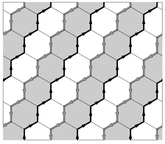
FIG. 4.: A ground-state configuration of fluxoids and superconducting currents at $f=1/2$ for the honeycomb network at low temperatures, in the London regime.

REFERENCES

- [1] See, for instance, ”Coherence in superconducting networks”, edited by J.E. Mooij and G.B.J. Schön, [Physica 152B, 1 (1988)].
- [2] B. Pannetier, J. Chaussy, and R. Rammal, J. Phys. (Paris) 44, L853 (1983).
- [3] B. Pannetier, J. Chaussy, R. Rammal, and J. C. Villegier, Phys. Rev. Lett. 53, 1845 (1984).
- [4] F. Nori and Q. Niu, Phys. Rev. B 37, 2364 (1988).
- [5] J.M. Gordon, A.M. Goldman, J. Maps, D. Costello, R. Tiberio, and B. Whitehead, Phys. Rev. Lett. 56, 2280 (1986).
- [6] R.G. Steinmann, B. Pannetier, Europhys. Lett. 5, 559 (1988).
- [7] M.G. Forrester, S.P. Benz and C.J. Lobb, Phys. Rev. B. 41, 8749 (1990).
- [8] A. Behrooz, et al., Phys. Rev. Lett. 57, 368 (1986); Phys. Rev. B 35, 8396 (1987).
- [9] G. S. Grest, P.M. Chaikin, and D. Levine, Phys. Rev. Lett. 60, 1162 (1988).
- [10] Y.-L. Lin and F. Nori, Phys. Rev. B 50, 15953 (1994).
- [11] See, for instance, B. Pannetier, J. Chaussy, R. Rammal, and J.C.Villegier, Phys. Rev. Lett. 53, 1845 (1984)
- [12] Y.-L. Lin and F. Nori, (2001), submitted to Phys. Rev. B, (accompanying paper).
- [13] W. Y. Shih and D. Stroud, Phys. Rev. B 32, 158 (1985).
- [14] M. S. Rzchowski, Phys. Rev. B 55, 11745 (1997).
- [15] Yi Xiao, Princeton Univ. Ph.D. thesis (2000).
- [16] M. J. Higgins, Y. Xiao, S. Bhattacharya, P.M.Chaikin, S.Sethuraman, R. Bojko and D. Spencer, Phys. Rev. B. 61, R894 (2000).
- [17] K. Park and D. A. Huse, Phys. Rev. B 64, 134522 (2001).
- [18] Yi Xiao, et al. (unpublished).
- [19] J. Vidal, R. Mosseri, and B. Douçot, Phys. Rev. Lett. 81, 5888 (1998).
- [20] C. C. Abilio, et al., Phys. Rev. Lett. 83, 5102 (1999).
- [21] M. F. Laguna, C. A. Balseiro, D. Dominguez and F. Nori, Phys. Rev. B 64, 104505 (2001).