[

Formation and rapid evolution of domain structure at phase transitions in slightly inhomogeneous ferroelectrics

Abstract

We present the first analytical study of stability loss and evolution of domain structure in inhomogeneous ferroelectric samples for exactly solvable model. The model assumes a short-circuited capacitor with two regions with slightly different critical temperatures $T_{c1}>T_{c2}$, where $T_{c1}-T_{c2}\ll T_{c1},T_{c2}$. Even a tiny inhomogeneity like $10^{-5}$K may result in splitting the system into domains below the phase transition temperature. At $T<T_{c2}$ the domain width $a$ is proportional to $(T_{c1}-T)/(T_{c1}-T_{c2})$ and quickly increases with lowering temperature. The minute inhomogeneities in $T_{c}$ may result from structural (growth) inhomogeneities which are always present in real samples and a similar role can be played by inevitable temperature gradients.

]

The idea that the phase transition in electroded short-circuited ferroelectric proceeds into homogeneous monodomain state[1] is very well known. Similar result also applies to free ferroelastic crystals. However, it has never been observed. Surprisingly, both electroded ferroelectrics and free ferroelastics do split into domains, although they should not. The present paper aims to answer why.

It is generally assumed that in the finite ferroelectric samples the domain structure appears in order to reduce the depolarizing electric field if there is a nonzero normal component of the polarization at the surface of the ferroelectrics [1, 2] (in complete analogy with ferromagnets [3]), if the field cannot be reduced by either conduction (usually negligible in ferroelectrics at low temperatures) or charge accumulation from environment at the surface [4]. On the other hand, in inhomogeneous ferroelastics (e.g. films on a substrate, or inclusions of a new phase in a matrix) the elastic domain structure accompanies the phase transition in order to minimize the strain energy, as is well understood in case of martensitic phase transformations [5] and epitaxial thin films [6, 7, 8].

In search for reasons of domain appearance in otherwise perfect electroded samples, which is not yet understood, we shall discuss a second order ferroelectric phase transition in slightly inhomogeneous electroded sample. This problem has not been studied before. We consider an exactly solvable case of a system, which has two slightly different phase transition temperatures in its two parts. While the phase transition occurs in the “soft” part of the system, the “hard” part may effectively play a role of a “dead” layer [10] and trigger a formation of the domain structure in the “soft” part with fringe electric fields penetrating the “hard” part. One has to check this possibility, but the behavior of the corresponding domain structure is expected to be unusual: it should strongly depend on temperature since further cooling transforms the “hard” part into a “soft” one, while the first “soft” part becomes “harder”. Since the inhomogeneity is small, one might expect that the domains would quickly grow with lowering temperature. We indeed find a rapid growth of the domain width linearly with temperature in the case of slightly inhomogeneous short-circuited ferroelectric. This behavior is generic and does not depend on particular model assumptions. Generally, the inhomogeneous ferroelectric systems pose various fundamental problems and currently attract a lot of attention. In particular, graded ferroelectric films and ferroelectric superlattices have been shown to have giant pyroelectric [11] and unusual dielectric response[12].

We shall consider the case of slightly inhomogeneous uniaxial ferroelectric in short-circuited capacitor that consists of two layers with slightly different critical temperatures, so that, for instance, a top part “softens” somewhat earlier than the bottom part does. We assume the easy axis $z$ perpendicular to electrode plates, and make use of the Landau free energy functional for given potentials on electrodes (zero in the present case)[9] $\tilde{F}=F_{LGD}\left[\vec{P}\right]+\int dV\left(-\vec{E}\vec{P}-\frac{E^{2}}{8\pi}\right),$ with

$$F_{LGD}[\vec{P}] = \sum_{p=1,2}\int dV[\frac{A_{p}}{2}P_{z}^{2}+\frac{B}{4}P_{z}^{4}$$ (2)

$$+\frac{D}{2}\left(\nabla_{\perp}P_{z}\right)^{2}+\frac{g}{2}\left(\partial_{z}P_{z}\right)^{2}+\frac{A_{\perp}}{2}\vec{P}_{\perp}^{2}],$$

where $P_{z}$ $\left(\vec{P}_{\perp}\right)$is the polarization component along (perpendicular to) the “soft” direction, index $p=1(2)$ marks the top (bottom) part of the film:

$$A_{1} = A,\qquad 0<z<l_{1},$$

$$A_{2} = A+\delta A,\qquad-l_{2}<z<0,$$

where $A_{1(2)}=\alpha(T-T_{c1(2)})$ and $\delta A>0$ (meaning $T_{c2}<T_{c1})$. The constant $\alpha=1/T_{0},$ where $T_{0}\sim T_{at}$ $(\sim T_{c})$ for displacive (order-disorder) type ferroelectrics.

The equation of state is $\delta F_{LGD}[P]/\delta\vec{P}=\vec{E}=-\nabla\varphi,$ where $\varphi$ is the electrostatic potential, or in both parts of the film $p=1,2:$

$$E_{z} = -\partial_{z}\varphi=A_{p}P_{z}+BP_{z}^{3}-D\nabla_{\perp}^{2}P_{z}-g\partial_{z}^{2}P_{z},$$ (3)

$$\vec{E}_{\perp} = A_{\perp}\vec{P}_{\perp},$$ (4)

These equations should be solved together with the Maxwell equation, ${\rm div}(\vec{E}+4\pi\vec{P})=0,$ or

$$\left(\partial_{z}^{2}+\epsilon_{a}\nabla_{\perp}^{2}\right)\varphi=4\pi\partial_{z}P_{z},$$ (5)

where the dielectric constant in the plane of the film is $\epsilon_{a}=1+4\pi/A_{\perp}.$

Loss of stability${\em.-}$ We shall now find conditions for loss of stability of the paraelectric phase close to $T_{c1}$ with respect to inhomogeneous polarization. At the point of stability loss the polarization is small and the nonlinear term $P_{z}^{3}$ must be omitted. We are looking for a nontrivial solution in a form of the ”polarization wave”,

$$P_{z},\varphi\propto e^{ikx}.$$ (6)

We shall check later that the stability will be lost for the wave vector $kl_{1}\gg 1,$ so that $\nabla_{\perp}^{2}P_{z}=k^{2}P_{z}\gg g\partial_{z}^{2}P_{z}\sim P_{z}/l_{1}^{2},$ and the last term in the right-hand side of (3) should be dropped. Going over to Fourier harmonics indicated by the subscript $k$, we obtain

$$\varphi_{k}^{\prime\prime}-\epsilon_{a}k^{2}\varphi_{k}=4\pi P_{zk}^{\prime},$$ (7)

where the prime indicates derivative $($ $f^{\prime}\equiv df/dz,$ $f^{\prime\prime}\equiv d^{2}f/dz^{2})$. We can exclude $P_{zk}$ with the use of the linearized equation of state (3), which gives

$$-\varphi_{k}^{\prime}=(A_{p}+Dk^{2})P_{zk}.$$ (8)

Substituting this into (7), we obtain $\varphi_{k}^{\prime\prime}-\frac{\epsilon_{a}k^{2}\left(A_{p}+Dk^{2}\right)}{4\pi}\varphi_{k}=0,$ where we have used $\left|A+Dk^{2}\right|/4\pi\ll 1,$ which is always valid in ferroelectrics. We shall see momentarily that the nontrivial solution appears only when $A_{1}+Dk^{2}<0,$ while $A_{2}+Dk^{2}>0.$ The resulting system is

$$\varphi_{1k}^{\prime\prime}+\chi_{1}^{2}k^{2}\varphi_{1k} = 0,$$ (9)

$$\varphi_{2k}^{\prime\prime}-\chi_{2}^{2}k^{2}\varphi_{2k} = 0,$$ (10)

where $\chi_{1}^{2}=-\frac{\epsilon_{a}\left(A_{1}+Dk^{2}\right)}{4\pi},$ $\chi_{2}^{2}=\frac{\epsilon_{a}\left(A_{2}+Dk^{2}\right)}{4\pi}.$ The boundary condition reads as

$$\frac{\varphi_{1k}^{\prime}}{A_{1}+Dk^{2}}=\frac{\varphi_{2k}^{\prime}}{A_{2}+Dk^{2}},$$ (11)

where we have used $\left|A_{1}+Dk^{2}\right|/4\pi\ll 1.$ We obtain from Eqs. (9)-(11) the condition for a nontrivial solution

$$\chi_{1}\tan\chi_{1}kl_{1}=\chi_{2}\tanh\chi_{2}kl_{2},$$ (12)

which has a homogeneous solution $k=0$ and the inhomogeneous solution with $k=k_{c}$ (14), hence we have to determine which one is actually realized. The inhomogeneous solution is easily found for $\chi_{2}kl_{2}\gtrsim 1,$ where $\tanh$ can be replaced by unity. Close to the transition $\chi_{2}/\chi_{1}\gg 1,$ and the solution is

$$\chi_{1}kl_{1}=\frac{\pi}{2}\frac{\chi_{2}kl_{1}}{1+\chi_{2}kl_{1}}\approx\frac{\pi}{2},$$ (13)

when $\chi_{2}kl_{1}\gg 1.$ This gives $|A|=Dk^{2}+\frac{\pi^{3}}{\epsilon_{a}k^{2}l_{1}^{2}}.$There is no solution for $\chi_{1}^{2}<0.$ The minimal value of $A$ for the nontrivial solution (onset of instability) is defined by

$$k_{c} = \left(\frac{\pi^{3}}{\epsilon_{a}Dl_{1}^{2}}\right)^{1/4}\approx\frac{\pi^{3/4}}{\epsilon_{a}^{1/4}}\frac{1}{\sqrt{d_{at}l_{1}}},$$ (14)

$$|A|_{c} = 2Dk_{c}^{2}=\frac{2\pi^{3/2}D^{1/2}}{\epsilon_{a}^{1/2}l_{1}}\approx\frac{2\pi^{3/2}}{\epsilon_{a}^{1/2}}\frac{d_{at}}{l_{1}},$$ (15)

where we have introduced the “atomic” size $d_{at}\sim\sqrt{D}$ comparable to the lattice parameter. We obtain the corresponding tiny shift in the critical temperature [see estimates below Eq.(17)] $T_{c1}-T_{c}\sim T_{0}d_{at}/\epsilon_{a}^{1/2}l_{1}.$ Hence, the system looses its stability very quickly below the bulk transition temperature. It is readily checked that the assumptions we used to obtain the solution are easily satisfied. Indeed, $\chi_{2}kl_{2}\gtrsim 1$ and $\chi_{2}kl_{1}\gg 1$ both correspond to approximately the same condition when $l_{1}\sim l_{2}:\delta A\gg\frac{4}{\pi^{1/2}\epsilon_{a}^{1/2}}\frac{d_{at}}{l_{1}},$ meaning that the difference between $T_{c}$ should be larger than the shift of $T_{c}$.

Now we have to determine when the transition into inhomogeneous state occurs prior to a loss of stability with respect to a homogeneous polarization. The homogeneous loss of stability corresponds to $A=A_{h}$ found from

$$A_{h}l_{1}+\left(A_{h}+\delta A\right)l_{2}=0.$$ (16)

For the inhomogeneous state to appear first, there must be $A_{c}>A_{h},$ or $\delta A>\frac{\pi^{3/2}(l_{1}+l_{2})}{\epsilon_{a}^{1/2}l_{1}}\frac{d_{at}}{l_{1}}.$ This means that very tiny inhomogeneity in the sample is enough to split it into the domain structure,

$$T_{c1}-T_{c2}=T_{0}\frac{\pi^{3/2}(l_{1}+l_{2})}{\epsilon_{a}^{1/2}l_{1}}\frac{d_{at}}{l_{1}},$$ (17)

which is estimated as $T_{at}\frac{d_{at}}{\epsilon_{a}^{1/2}l_{1}}\lesssim\epsilon_{a}^{-1/2}(10^{4}-10^{5})10^{-7}K=(10^{-3}-10^{-2}){\rm K}$ for displacive systems, and $T_{c}\frac{d_{at}}{\epsilon_{a}^{1/2}l_{1}}\lesssim\left(10^{-5}-10^{-4}\right)$K for order-disorder systems. Certainly, such a small temperature and/or compositional inhomogeneity exists in all usual experiments.

Domain structure at $T_{c2}<T<T_{c1}$ $(A<0,$ $A+\delta A>0).-$ After stability loss the resulting ”polarization wave” quickly develops into a domain structure, as we shall now demonstrate. In the region well below $T_{c1}$ we can use the linearized equation of state

$$E_{z}=(A+3BP_{01}^{2})(P_{z}-P_{01})=-2A(P_{z}-P_{01}),$$ (18)

where $\left|P_{01}\right|=\sqrt{-A/B}$ is the spontaneous polarization in the top layer, which gives $P_{z1}=P_{01}+\frac{1}{2|A|}E_{z}$, $P_{z2}=\frac{1}{A_{2}}E_{z},$ for the top and bottom layers, respectively. In this case the equation for the potential $\varphi$ (5) reduces to a standard Laplace equation $\left(\epsilon_{c}\partial_{z}^{2}+\epsilon_{a}\nabla_{\perp}^{2}\right)\varphi=0,$ with the boundary condition

$$\epsilon_{c1}\partial_{z}\varphi_{1}-\epsilon_{c2}\partial_{z}\varphi_{2}=4\pi P_{01}(x),$$ (19)

where $\epsilon_{c1}=1+2\pi/|A|,$ $\epsilon_{c2}=1+4\pi/A_{2}.$

The spontaneous polarization in the top layer alternates from domain to domain as $P_{01}(x)=\pm\left|P_{01}\right|\equiv\pm\sqrt{-A/B}.$ We are looking for a solution in a form of a domain structure with a period $T=2a$ (Fig. 1),

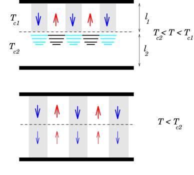
FIG. 1.: Schematic of the domain structure with the period $2a$ in inhomogeneous ferroelectric film of the thickness $l_{1}+l_{2}$. Top and bottom layers have slightly different critical temperatures $T_{c1}>T_{c2}$, $T_{c1}-T_{c2}\ll T_{c1},T_{c2}$. Slightly below $T_{c1}$ the top layer splits into domains with electric fringe field propagating into the bottom layer (fringe field shown as the hatched area in the top panel). The domains persist and evolve below $T_{c2}$ when both layers exhibit a ferroelectric (or ferroelastic) transition (bottom panel).

$$P_{01}(x)=\sum_{k}P_{01k}e^{ikx},\hskip 14.45377pt\varphi(x)=\sum_{k}\varphi_{k}e^{ikx},$$ (20)

with $k\equiv k_{n}=2\pi n/T=\pi n/a,$ $n=\pm 1,\pm 2,...$ Going over to the Fourier harmonics, we can write the Laplace equations for both parts of the film as

$$\epsilon_{c1}\varphi_{1k}^{\prime\prime}-\epsilon_{a}k^{2}\varphi_{1k} = 0,$$ (21)

$$\epsilon_{c2}\varphi_{2k}^{\prime\prime}-\epsilon_{a}k^{2}\varphi_{2k} = 0,$$ (22)

with the boundary conditions at the interface $z=0$

$$\varphi_{1k}=\varphi_{2k},\qquad\epsilon_{c1}\varphi_{1k}^{\prime}-\epsilon_{c2}\varphi_{2k}^{\prime}=4\pi P_{01k}$$ (23)

The corresponding electrostatic (stray) field part of the energy is found as [10] $\tilde{F}_{es}=\frac{1}{2}\int d{\cal A}\sigma_{s}\varphi\left(z=0\right),$ where $\sigma_{s}$ is the density of bound charge at the interface , corresponding to only the spontaneous part of the polarization $P_{01}(x),$ and integration goes over the area ${\cal A}$ between two parts of the film. We calculate this expression by going over to Fourier expansion (20) and using the fact that in the present geometry $\sigma_{s}(x)=-P_{01}(x)$ (and, therefore, its Fourier component $\sigma_{sk}=-P_{01k}),$

$$\frac{\tilde{F}_{es}}{{\cal A}}=\sum_{k>0}\frac{4\pi|P_{01k}|^{2}}{kD_{k}},$$ (24)

$D_{k}=\epsilon_{a}^{1/2}\left[\epsilon_{c1}^{1/2}\coth\sqrt{\frac{\epsilon_{a}}{\epsilon_{c1}}}kl_{1}+\epsilon_{c2}^{1/2}\coth\sqrt{\frac{\epsilon_{a}}{\epsilon_{c2}}}kl_{2}\right],$ with $k=\pi n/a,$ $n=1,2,...,$ similar to [13]. Note that here $P_{01k}=2\left|P_{01}\right|/i\pi n,$ $n=2j+1,$ $j=0,1,...$ and zero otherwise. Adding the surface energy of the domain walls, we obtain the free energy of the domain pattern

$$\frac{\tilde{F}}{{\cal A}}=\frac{\gamma_{1}l_{1}}{a}+\frac{16P_{01}^{2}a}{\pi^{2}}\sum_{j=0}^{\infty}\frac{1}{\left(2j+1\right)^{3}D_{2j+1}},$$ (25)

where $D_{n}=D_{k_{n}}.$ Not very close to $T_{c}$ the argument of $\coth$ is $\sqrt{\frac{\epsilon_{a}}{\epsilon_{c1}}}kl_{1}\gtrsim 1,$ so that $D_{k}=\epsilon_{a}^{1/2}\left(\epsilon_{c1}^{1/2}+\epsilon_{c2}^{1/2}\right).$ Minimizing the free energy, we find the domain width

$$a=\left[\frac{\pi^{2}\epsilon_{a}^{1/2}\left(\epsilon_{c1}^{1/2}+\epsilon_{c2}^{1/2}\right)}{14\zeta(3)}\Delta_{1}l_{1}\right]^{1/2},$$ (26)

where $\Delta_{1}\equiv\gamma_{1}/P_{01}^{2}=d_{at}|A|^{1/2}$ is the characteristic microscopic length, and $d_{at}\equiv\frac{2^{3/2}}{3}D^{1/2}$ is comparable to a lattice spacing (“atomic” length scale). The expression (26) is valid when $\sqrt{\frac{\epsilon_{a}}{\epsilon_{c1}}}kl_{1}\gtrsim 1,$ or $|A|\gtrsim 2d_{at}/\left(\pi\epsilon_{a}^{1/2}l_{1}\right),$ meaning that one has to be below $T_{c}$ by a tiny amount $T_{c1}-T\gtrsim T_{0}d_{at}/\left(\epsilon_{a}^{1/2}l_{1}\right),$ estimated earlier. Note that close to $T_{c1}$ one obtains for the domain width

$$a=a_{K}\equiv\left[\frac{\pi^{5/2}\epsilon_{a}^{1/2}}{7\sqrt{2}\zeta(3)}d_{at}l_{1}\right]^{1/2},$$ (27)

and this value does not depend on temperature. We shall formally refer to this result as the Kittel domain width.

Incidentally, close to $T_{c2}$ the domain width is $a\approx\left[\frac{\pi^{2}\epsilon_{a}^{1/2}\epsilon_{c2}^{1/2}}{14\zeta(3)}\Delta_{1}l_{1}\right]^{1/2}\propto\epsilon_{c2}^{1/4},$ which formally diverges $\propto\left(T-T_{c2}\right)^{-1/4}.$ However, in the vicinity of $T_{c2}$ the induced polarization in the formerly “hard” part has about the same value as the spontaneous polarization in the “soft” part, $P_{z2}\approx P_{01}.$ Then the equation of state in the bottom part becomes strongly non-linear, since the cubic term is much larger than the linear term, $BP_{z2}^{3}\approx BP_{01}^{3}=AP_{01}\approx AP_{z2}\gg A_{2}P_{z2}$, in the equation of state (since $A\gg A_{2}$ close to $T_{c2})$, so the response of the bottom layer does not actually soften in this region. In this case our derivation does not apply, but it is practically certain that the domain structure in the vicinity of $T_{c2}$ would evolve continuously upon cooling, Fig. 2.

Domain structure at low temperatures ($T<T_{c2},$ $A<0,$ $A+\delta A<0).-$ When the system is cooled to below the critical temperature $T_{c2}$, a spontaneous polarization $\left|P_{02}\right|=\sqrt{-A_{2}/B}$ also appears in the bottom layer. The domain structure simultaneously develops in the whole crystal with domain walls running parallel to the ferroelectric axis through the whole crystal (if they were discontinuous at the interface between the two parts of the crystal this would have created a large depolarizing electric field). The electrostatic energy requires a solution of the same Laplace equations (21) and (22), only the boundary condition (23) would now read

$$\epsilon_{c1}\varphi_{1k}^{\prime}-\epsilon_{c2}\varphi_{2k}^{\prime}=4\pi(P_{01k}-P_{02k}),$$ (28)

where $\epsilon_{c1(2)}=1+2\pi/|A_{1(2)}|\approx 2\pi/|A_{1(2)}|.$ Note that the density of the bound charge at the interface, corresponding to this discontinuity of spontaneous polarization, is now $\sigma_{k}=-(P_{01k}-P_{02k}).$ Therefore, we immediately obtain for the total free energy of the structure, analogously to the previous case (25),

$$\frac{\tilde{F}}{{\cal A}} = \frac{P_{01}^{2}\Delta_{1}l_{1}+P_{02}^{2}\Delta_{2}l_{2}}{a}$$ (30)

$$+\frac{16(P_{01}-P_{02})^{2}a}{\pi^{2}}\sum_{j=0}^{\infty}\frac{1}{\left(2j+1\right)^{3}D_{2j+1}},$$

where $\Delta_{1(2)}=d_{at}\sqrt{|A_{1(2)}|}.$ Not very close to $T_{c2}$ we would have $\sqrt{\frac{\epsilon_{a}}{\epsilon_{c2}}}kl_{2}\gtrsim 1,$ and the minimum of the free energy $\tilde{F}$ is achieved for the domain width

$$a = \frac{1}{1-P_{02}/P_{01}}$$ (31)

$$\times \left[\frac{\pi^{2}\epsilon_{a}^{1/2}\left(\epsilon_{c1}^{1/2}+\epsilon_{c2}^{1/2}\right)}{14\zeta(3)}\left(\Delta_{1}l_{1}+\Delta_{2}l_{2}\frac{P_{02}^{2}}{P_{01}^{2}}\right)\right]^{1/2}.$$ (32)

Close to the critical point $T_{c2}$ the domain width formally behaves as $a\propto\epsilon_{c2}^{1/4}\propto(T_{c2}-T)^{-1/4}$, as found just above $T_{c2}$ before. The same argument indicates though that our derivation does not apply in this region, but non-linearity should not cause a substantial change in the domain structure.

With lowering the temperature to the region where $|A|\gg\delta A,$ we will have $P_{02}/P_{01}=\sqrt{(A+\delta A)/A}\approx 1+\delta A/2A,$ so that $1-P_{02}/P_{01}\approx 2|A|/\delta A\gg 1$ becomes a large prefactor. Note that in this region $\epsilon_{c1}\approx\epsilon_{c1}=2\pi/|A|,$ $\Delta_{1}\approx\Delta_{2}=d_{at}\sqrt{|A|},$ and the domain width evolves as

$$a=\frac{|A|}{\delta A}\left[\frac{2^{5/2}\pi^{5/2}\epsilon_{a}^{1/2}}{7\zeta(3)}d_{at}(l_{1}+l_{2})\right]^{1/2},$$ (33)

It becomes much larger than the Kittel width,

$$\frac{a}{a_{K}}=2^{3/2}\left(\frac{l_{1}+l_{2}}{l_{1}}\right)^{1/2}\frac{T_{c1}-T}{T_{c1}-T_{c2}}\gg 1,$$ (34)

growing linearly with lowering temperature, if the pinning of the domain walls is negligible (Fig. 2).

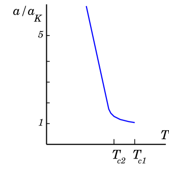
FIG. 2.: The domain width in slightly inhomogeneous ferroelectric or ferroelastic in the units of $a_{K}$, the Kittel width (27). $a=a_{K}$ when the domain structure sets in at $T\approx T_{c1}$, and then it grows linearly with the temperature to large values $a\gg a_{K}$.

Close to the lower critical point the linearized equation of state does not apply but the response of the bottom layer remains finite, and we expect, as mentioned above, that the domain structure would evolve rather gradually across $T_{c2}$, Fig. 2.

Summarizing, in a ferroelectric sample with a tiny inhomogeneity of either the critical temperature or temperature itself (i.e. in the presence of a slight temperature gradient and/or minute compositional inhomogeneity across the system) the domain structure abruptly sets in when the spontaneous polarization appears in the softest part of the sample (i.e. the part with maximal $T_{c}$). This takes place when the difference in $T_{c}$ in the parts of the sample is just $(10^{-3}-10^{-2}){\rm K}$ for displacive systems, and even smaller, $\left(10^{-5}-10^{-4}\right)$K, for order-disorder systems. The period of the structure then grows linearly with lowering temperature and quickly becomes much larger than the corresponding Kittel period.

This result does not depend on specific geometry assumed in the present model. Indeed, if local $T_{c}=T_{c}(z)$ varies continuously, like in graded ferroelectrics [11], it can be approximated by a piece-wise distribution of a sequence of “slices”. Upon cooling the system first looses stability in the softest part of thickness $l_{s},$ which is derived from the position of the boundary where local $T_{c}=0,$ with respect to a domain structure with fine period $\propto\sqrt{l_{s}}.$ The domains extend into the bulk of the system and become wider with further cooling, since $l_{s}$ increases. In electroded sample there will be no branching and domain walls would run straight across all transformed slices. Otherwise, discontinuities would have resulted in very strong depolarizing field. If the overall inhomogeneity is small, the picture would obviously remain very similar to the two-slice model solved above. The same arguments remain valid if the inhomogeneity were to have more complex form/distribution in a sample. The novel feature of the present effect of the depolarizing field is that it appears not due to surface charges, which are screened out by the electrodes, but because of the bulk inhomogeneity. The bulk depolarizing fields are present in other important classes of inhomogeneous ferroelectrics, graded ferroelectric films[11] and superlattices of different ferroelectrics (e.g. KNbO₃/KTaO${}_{3})$[12], and may be responsible for their unusual behavior.

We have shown that a very tiny temperature gradient, or a slight compositional inhomogeneity, etc., would result in practically any crystal eventually splitting into domains no matter how high the quality of it is. The unusual evolution of the domain pattern, found in the present paper, when it starts from very fine domains at $T_{c}$ and then grows linearly with temperature to very large sizes, has been reported in Ref. [14] for $\sim 1$mm thick TGS crystals. It is worth noting that the result is very general and applies also to slightly inhomogeneous free ferroelastic crystals[15]. Other implications include extensively studied graded films and ferroelectric superlattices[11, 12]. It would be very interesting to perform controlled experiments for the domain structure close to the phase transition to check the present theory.

REFERENCES

• [1] V.L. Ginzburg, Usp. Fiz. Nauk 38, 490 (1949).
• [2] W. Känzig, Phys. Rev. 87, 385 (1952); T. Mitsui and J. Furuichi, Phys. Rev. 90, 193 (1953).
• [3] L.D. Landau and E.M. Lifshitz, Electrodynamics of Continuous Media (Butterworth Heinemann, Oxford, U.K., 1980), Sec 44.
• [4] F. Jona and G. Shirane, Ferroelastic Crystals (Pergamon, Oxford, 1962), Ch. 3.
• [5] A.G. Khachaturyan, Theory of Structural Transformations in Solids (John Wiley, New York, 1983).
• [6] A.L. Roitburd, Phys. Status Solidi A 37, 329 (1976).
• [7] A.M. Bratkovsky and A.P. Levanyuk, Phys. Rev. Lett. 86, 3642 (2001).
• [8] A.M. Bratkovsky and A.P. Levanyuk, Phys. Rev. B 64, 134107 (2001).
• [9] Ref.[3], Secs. 10 and 19.
• [10] A.M. Bratkovsky and A.P. Levanyuk, Phys. Rev. Lett. 84, 3177 (2000).
• [11] N.W. Schubring et al., Phys. Rev. Lett. 68, 1778 (1992); F. Jin et al., Appl. Phys. Lett. 73, 2838 (1998); M. Brazier et al., Appl. Phys. Lett. 72, 1121 (1998).
• [12] J. Sigman et al., Phys. Rev. Lett. 88, 097601 (2002).
• [13] A.M. Bratkovsky and A.P. Levanyuk, Phys. Rev. B 63, 132103 (2001).
• [14] N. Nakatani, Jap. J. Appl. Phys. 24, L528 (1985).
• [15] A.M. Bratkovsky and A.P. Levanyuk, to be published.