Quasiequilibrium sequences of synchronously rotating binary neutron stars with constant rest masses in general relativity
— Another approach without using the conformally flat condition —

Abstract

We have computed quasiequilibrium sequences of synchronously rotating compact binary star systems with constant rest masses. This computation has been carried out by using the numerical scheme which is different from the scheme based on the conformally flat assumption about the space.

Stars are assumed to be polytropes with polytropic indices of $N=0.5$, $N=1.0$, and $N=1.5$. Since we have computed binary star sequences with a constant rest mass, they provide approximate evolutionary tracks of binary star systems. For relatively stiff equations of state ($N<1.0$), there appear turning points along the quasiequilibrium sequences plotted in the angular momentum — angular velocity plane. Consequently secular instability against exciting internal motion sets in at those points. Qualitatively, these results agree with those of Baumgarte et al. who employed the conformally flat condition.

We further discuss the effect of different equations of state and different strength of gravity by introducing two kinds of dimensionless quantities which represent the angular momentum and the angular velocity. Strength of gravity is renormalized in these quantities so that the quantities are transformed to values around unity. Therefore we can clearly see relations among quasiequilibrium sequences for a wide variety of strength of gravity and for different compressibility.

I Introduction

Binary neutron stars are very interesting objects. From the observational point of view, we will have a chance to get new eyes for the Universe by detecting gravitational waves in the first or second decade of this century. It is highly possible that the first signal may be that from compact binary stars, such as binary neutron stars, a black hole — neutron star binary system, or binary black holes. On the other hand, theoretically, our understanding of evolution of compact binary stars is far from complete because it is considerably difficult to treat the “2-body” problem from a state with a wide separation to a merging stage consistently in the framework of general relativity.

However, recent investigations have found a new approach to this problem. Since the time scale of the orbital change due to gravitational wave emission is rather long compared with the orbital period except for in the final few milliseconds of the coalescing stage, we can neglect gravitational wave emission for most stages of evolution. In other words, we can treat the system in “quasiequilibrium” (see e.g., WMM96 ; BCSST98a ; BGM99 ).

Following this idea, several groups have obtained quasiequilibrium sequences of binary neutron stars WMM96 ; BCSST98a ; BGM99 ; UE00 ; UUE00 . Most of them adopted the assumption that the spatial part of the metric is conformally flat (the conformally flat condition: hereafter, CFC) WMM96 ; BCSST98a ; BGM99 ; UE00 . For axisymmetric rotating polytropes results of the scheme with the CFC were compared with those obtained by the numerically exact code and found to be reasonably accurate CST96 . However, since there are no exact numerical solutions for binary configurations, one could not know the accuracy of the results obtained by the scheme with the CFC.

Therefore, it is desirable to develop different schemes from that with the CFC and to compare results of different schemes for nonaxisymmetric configurations. As one of those alternatives, in the previous paper, we developed a new numerical scheme to obtain quasiequilibrium structures of nonaxisymmetric compact stars as well as the space time around those stars in general relativity and obtained quasiequilibrium sequences of synchronously rotating binary polytropes UUE00 . In that scheme, the Einstein equations are solved directly without assuming the CFC. The obtained results, however, could not be compared with those of BCSST98a because different polytropic relations were used.

In this paper, we have used the same polytropic equation as that used in BCSST98a and computed quasiequilibrium sequences of synchronously rotating polytropes with a constant rest mass. Therefore, we can directly compare our results with those with the CFC. In actual computations, we have improved our numerical scheme and succeeded in making our scheme more robust.

II Assumptions and basic equations

II.1 Assumptions

As mentioned in Introduction, we can neglect the effect of gravitational wave emission for almost all stages except for the last few milliseconds of the coalescence of binary systems and choose a rotating frame in which the system is in a stationary state.

In this paper, we use the units of $c=G=1$ except for in the final section and we will make the following assumptions (see, Usui, Uryū, and Eriguchi UUE00 for a more detail):

(1)

We deal with a binary system which consists of two stars of equal masses in a circular orbit.

(2)

The binary star system is in a stationary state in the rotating frame with the orbital angular velocity $\Omega$.

(3)

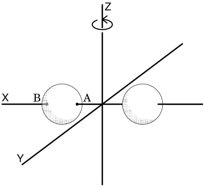
Figure 1: Schematic view of the binary system and the coordinates. The $x$ axis is set along the line joining the two centers of mass of the two stars and the origin is set at their midpoint. The $z$ axis is along the rotation axis. Points A, B are set at the intersections of the surface of the star and the $x$ axis. The inner intersection is point A and the outer one is point B.

Axes of spins of two stars and that of the orbital motion are parallel to one another. A schematic figure of the system is shown in Fig. 1.

(4)

Spins of two stars are synchronized to the orbital motion. Each star is rigidly rotating with the angular velocity $\Omega$ if seen from a distant place.

(5)

The matter of the star is a perfect fluid and the equation of state for the matter is assumed to be polytropic:

$$p = K\rho^{1+1/N}\ ,$$ (1)

$$\varepsilon = \rho+Np\ ,$$ (2)

where $p$, $\rho$, $\varepsilon$, $N$, and $K$ are the pressure, the rest mass density, the energy density, the polytropic index, and the polytropic constant, respectively.

II.2 Metric and basic equations

In addition to the assumptions mentioned above, we further assume the following form for the metric in the spherical coordinates $(r,\theta,\varphi)$ :

$$ds^{2}=-e^{2\nu}dt^{2}+r^{2}\sin^{2}\theta e^{2\beta}(d\varphi-\omega dt)^{2}+e^{2\alpha}dr^{2}+r^{2}e^{2\alpha}d\theta^{2}\ ,$$ (3)

where $\nu$, $\beta$, $\omega$, and $\alpha$ are the metric potentials which are functions of $r$, $\theta$, and $\varphi$. Although this form of the metric becomes exact for stationary axisymmetric configurations, it is not exact for nonaxisymmetric configurations. Therefore, it must be extended to a more general form in the future.

The Einstein equations with appropriate boundary conditions can be written down for the metric form Eq. (3), and are transformed to integral representations by using the Green function for the Laplacian in the flat space (see UUE00 ). Here we solve four equations for the metric potentials, $\nu$, $\beta$, $\omega$, and $\alpha$, and the rest of the Einstein equations are not used. In the concrete, we do not consider ${(t)(r)}$, ${(t)(\theta)}$, ${(r)(\varphi)}$, and ${(\theta)(\varphi)}$ components of the Einstein equations (see UUE00 ). We can check how these equations are satisfied or violated after obtaining the solutions to the rest of the Einstein equations. In actual computations, even for highly relativistic configurations, these equations are satisfied quite well, to within $0.5\%$, if we estimate the relative errors by the following quantity:

$$\frac{R_{(\mu)(\nu)}-8\pi\left(T_{(\mu)(\nu)}-1/2g_{(\mu)(\nu)}T\right)}{\sum{\Bigl{|}\mbox{each term of }R_{{(\mu)}{(\nu)}}\Bigr{|}}}\ ,$$ (4)

where $R_{(\mu)(\nu)},T_{(\mu)(\nu)}$ and $T$ are the Ricci tensor, the energy momentum tensor and the trace of the energy momentum tensor, respectively. It must be noted that for nonaxisymmetric quasiequilibrium configurations it is impossible to satisfy all components of the Einstein equations because there cannot exist “exact” quasiequilibrium configurations as far as the asymptotic flat condition is assumed.

III Method of calculations

III.1 Solving scheme

The method of calculation is almost the same as that used in the previous paper UUE00 except for several improvements. We will briefly summarize the scheme and explain the improved changes in some detail.

We solve the hydrostatic equation and the metric potentials iteratively by adopting the HSCF (Hachisu’s Self-Consistent Field) method UUE00 ; H86 ; KEH89 . In particular, as mentioned before, the Einstein equations for the metric are transformed into the integral equations by constructing the Laplacian in the flat space. In this procedure we have to add the following derivative to both sides of the equation:

$$\frac{1}{r^{2}\sin^{2}\theta}\frac{\partial^{2}g_{{\mu}{\nu}}}{\partial\varphi^{2}}\ .$$ (5)

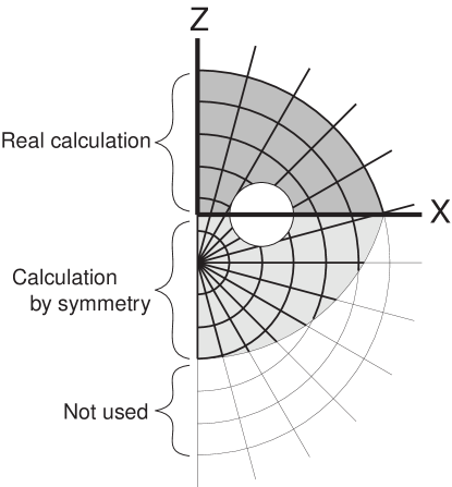
Figure 2: Shifted coordinate system. A circle located on the $x$-axis denotes a component star of the binary.

This term may cause the iteration diverge because, once a certain amount of numerical errors is introduced by chance, this error may not decrease but increase iteration by iteration near the coordinate center. To avoid this problem, we have shifted the coordinate center downwards along the $z$-axis as Fig. 2. Numerical computations are carried out only in the upper half of the whole space, i.e., above the equatorial plane of the binary star systems, and quantities in the lower half are computed by making use of the symmetry of the physical quantities about the equatorial plane. Consequently, it is noted that 25% of the whole grid points is used in the actual calculations. As shown later, this scheme works nicely.

We have used $(r\times\theta\times\varphi)=(200\times 119\times 81)$ grid points for ($0\leq\tilde{r}\leq 2.0$, $0\leq\theta\leq\pi$, $0\leq\varphi\leq\pi/2$), where $\tilde{r}=r/r_{B}$, and $r_{B}$ means the distance from the orbital axis to point B (see Fig. 1).

III.2 Physical quantities

Since there exist no exact equilibrium or stationary states for real compact binary stars with a flat space at infinity, it is difficult to define exactly the conserved quantities for nonaxisymmetric configurations in general relativity. However, for an asymptotically flat spacetime, we can define the approximate total angular momentum, $J_{\rm tot}$, and the approximate total gravitational mass, $M_{\rm tot}$, as:

$$J_{\rm tot} = \int r\sin\theta e^{2\alpha+2\beta}\frac{(\varepsilon+p)v}{1-v^{2}}r^{2}\sin\theta drd\theta d\varphi$$ (6)

$${}+\frac{1}{4\pi}\int e^{2\alpha}\frac{v}{r\sin\theta}\left[\frac{\partial^{2}\alpha}{\partial\varphi^{2}}+\frac{\partial\alpha}{\partial\varphi}\left(\frac{\partial\alpha}{\partial\varphi}-\frac{\partial\beta}{\partial\varphi}-\frac{\partial\nu}{\partial\varphi}\right)\right]r^{2}\sin\theta drd\theta d\varphi\ ,$$

$$M_{\rm tot} = \int e^{2\alpha+\beta+\nu}\left\{(\varepsilon+p)\frac{1+v^{2}}{1-v^{2}}+2p\right\}r^{2}\sin\theta drd\theta d\varphi$$ (7)

$${}+\int 2r\sin\theta e^{2\alpha+2\beta}(\varepsilon+p)\frac{v\omega}{1-v^{2}}r^{2}\sin\theta drd\theta d\varphi\ ,$$

where $v=r(\Omega-\omega)\sin\theta e^{\beta-\nu}$ is the velocity of the matter. These expressions can be obtained by making use of the behaviors of the metric functions at flat infinity as follows (see UUE00 for a more detail):

$$\omega\sim 2J_{\rm tot}/r^{3}\ ,\ \partial\omega/\partial r\sim-6J_{\rm tot}/r^{4}\ ,\ \partial{\nu}/\partial{r}\sim{M_{\rm tot}}/{r^{2}},\ {\rm at}\ r\sim\infty\ .$$ (8)

Notice that these expressions are not general forms and different from the ADM quantities used in Baumgarte et al. BCSST98a . To compare our results with those with the CFC, it would be desirable to employ the same definitions of physical quantities as theirs. For conformally flat situations, the ADM mass can be easily evaluated by using the matter contribution in addition to the contribution of the extrinsic curvatures as seen in Baumgarte et al.  BCSST98a . With our choice of the metric (Eq. (3)), however, it is difficult to use the same definition because we do not use the conformal factor. Therefore we follow the scheme used by Bardeen B73 and derive the total mass and the total angular momentum by considering the asymptotic behavior of the 4-metric. In the previous paper UUE00 , the expression of the angular momentum (Eq.(48) in UUE00 ) was incorrect. Numerical values of the angular momentum in UUE00 contain about $15\%$ errors at maximum due to that wrong expression.

On the other hand, for the rest mass, it is natural to define as:

$$M_{\rm 0,tot} = \int\rho u^{t}\sqrt{-g}\cdot r^{2}\sin\theta drd\theta d\varphi$$ (9)

$$= \int e^{2\alpha+\beta}\rho\frac{1}{\sqrt{1-v^{2}}}r^{2}\sin\theta drd\theta d\varphi\ .$$

Since we use the same polytropic relation as that used by Baumgarte et al. BCSST98a , we can choose the same nondimensional quantities as they did by using the polytropic constant $K$ and the polytropic index $N$ as:

$$M = K^{N/2}\bar{M}\ ,$$ (10)

$$M_{0} = K^{N/2}\bar{M_{0}}\ ,$$ (11)

$$\varepsilon = K^{-N}\bar{\varepsilon}\ ,$$ (12)

$$\Omega = K^{-N/2}\bar{\Omega}\ ,$$ (13)

$$J = K^{N}\bar{J}\ ,$$ (14)

where $M$, $M_{0}$ and $J$ are the gravitational mass, the rest mass and the angular momentum of a component star and quantities with “bar” mean nondimensional ones.

III.3 Model parameters

For polytropes, the equation of state is fixed by choosing one parameter, constant $K$, in addition to the polytropic index $N$. After the equation of state is fixed, we need to specify two more parameters to determine one rotating equilibrium configuration: one represents the strength of gravity and the other for the rotation. In our formulation, we choose the following two parameters:

(1)

The maximum energy density, $\varepsilon_{c}$.

(2)

The ratio of the shortest distance $r_{A}$ (distance from the orbital axis to point A, see Fig. 1) to the largest distance $r_{B}$ (distance from the orbital axis to point B, see Fig. 1), $q$:

$$q\equiv\frac{r_{A}}{r_{B}}\ .$$ (15)

This quantity $q$ indirectly specifies the rotational state and is related to the separation — distance between the two stars — as $d=r_{B}(1+q)$, where $d$ is the distance between the geometrical centers of the stars.

Since the quantity $K$ does not appear in the basic equations due to our normalization, i.e., Eqs. (10)–(14), we can treat the problem by specifying only three parameters, $\varepsilon_{c}$ (or nondimensional quantity $\bar{\varepsilon}_{c}$) and $q$, in addition to the polytropic index $N$.

IV Results

IV.1 Construction of evolutionary sequences of binaries with constant rest masses

In order to consider realistic evolutions of compact binary star systems, it would be important to find conserved quantities which characterize the evolution. Although, during evolutions of binary neutron star systems, the gravitational mass and the angular momentum are lost from the system, the baryon number of the system should be conserved because we do not consider the mass loss or the Roche lobe overflow. Therefore a sequence of a constant rest mass (baryon mass) can be considered to provide an evolutionary track.

Even if the rest mass of the star is specified, one cannot follow an evolutionary sequence of binary stars. One needs to know the following two things: 1) the change of the equation of state and 2) the change of the velocity field of the stars. Concerning the first point, as far as one uses the polytropic relations, it is impossible to know the change of the equation of state. Thus we adopt the same approximation as Baumgarte et al. did, i.e., the polytropic index $N$ and the constant $K$ are fixed during binary evolutions BCSST98a . Concerning the value of $K$, it may be a reasonable assumption because $K$ means the entropy in the Newtonian limit and the evolution can be treated as an almost adiabatic process, i.e., the timescale of viscous heating is much longer than evolutionary time scale due to the back reaction of gravitational wave emission.

As for the second point, it is widely believed that binary neutron star systems evolve irrotationally K92 ; BC92 . However, since the purpose of the present paper is to present an alternative method of solving binary neutron stars without employing the CFC, we assume that the system evolves by keeping synchronous rotation, although its evolution is not realistic.

Although our final goal in this paper is to obtain evolutionary sequences of constant rest masses for the specified polytropic relation, it is not easy to follow constant rest mass sequences because the rest mass is not a local quantity but a global quantity which can be computed after the structure of the binary star is obtained. Thus, we construct evolutionary sequences of constant rest masses by the following procedure:

(1)

Fix the polytropic index $N$.

(2)

Calculate sequences by changing $\bar{\varepsilon}_{c}$ for a fixed value of $q$. After obtaining the structure, compute global physical quantities such as the rest mass, the gravitational mass, and the angular momentum.

(3)

Repeat Step (2) by changing the value of $q$.

(4)

Specify one value of the rest mass and interpolate physical quantities with different values of $q$ for the specified rest mass by using quantities obtained in Steps (2)-(3). Thus constant rest mass sequences are obtained.

(5)

Change the rest mass and repeat Step (4) and construct sequences for different strength of gravity.

Hereafter, we choose the compactness, $(M/R)_{\infty}$, as the parameter of the strength of gravity. Here $M_{\infty}$ and $R_{\infty}$ are the gravitational mass and the Schwarzschild radius of a spherical star with the same value of the rest mass as that of the sequence which we consider.

IV.2 Numerical results

IV.2.1 $N=1.0$ sequences

In Fig. 3, the nondimensional rest mass of each star is plotted against the nondimensional central energy density. Each curve represents a sequence along which the separation $q$ is fixed but the energy density $\bar{\varepsilon}_{c}$ is varied. Seven curves correspond to the sequences of $q=0.00$ (contact), $0.05$, $0.10$, $0.15$, $0.20$, $0.25$, and $0.30$. From this figure, we can see that as the central energy density increases, the rest mass increases until a certain critical point. However, as the density increases further, the mass begins to decrease because of the general relativistic effect. The curves at the upper side correspond to the binary sequences with smaller separations and the uppermost curve denotes the sequence at the contact phase. For larger separations, each star can be considered to approach the spherical configuration.

By using the information in this figure, we can consider evolutionary sequences with constant rest masses because horizontal lines can be regarded as such sequences. Thus, we choose four evolutionary sequences of four constant rest masses which correspond to four different compactnesses, i.e., $(M/R)_{\infty}=0.05$, $0.10$, $0.15$, and $0.20$.

The energy density contours for selected models at the contact phase are shown in Fig. 4. In this figure, equidensity contours are drawn for several $N$ and $(M/R)_{\infty}$.

In Fig. 5, the nondimensional angular velocity is plotted against the nondimensional angular momentum. Four curves correspond to sequences with the compactness mentioned above. As the angular momentum decreases due to gravitational wave emission, the binary system evolves to the upper-left direction along the curve. If the curve has a turning point, the system becomes secularly unstable at that point. As seen from this figure, for $N=1.0$ polytropes, it is very difficult to tell whether turning points appear or not, because turning points, if exist, seem to coincide with the contact states.

In this same figure, the results of Baumgarte et al. BCSST98a are also plotted by using several different types of symbols. If we assume that the turning points coincide with the contact points, we can see almost the same tendency about the occurrence of secular instability, although the values are not the same. While Baumgarte et al. BCSST98a used the ADM quantities, we have introduced our approximate definitions as mentioned in Sec. III.2. Although these quantities coincide in the Newtonian limit, the slight differences appear for highly relativistic, highly nonlinear configurations.

Fig. 6 shows the nondimensional central energy density $\bar{\varepsilon}_{c}$ — separation parameter $q$ relation. From this figure, we can see that the central energy density decreases as the orbit shrinks, i.e., as the evolution proceeds. The central energy density seems to decrease as the separation become larger, too. However, this may not be real because, as mentioned before, a small number of grid points cover the matter region and values cannot be highly accurate. Thus, there is no tendency to collapse individually prior to merging, which was suggested by Wilson et al. WMM96 .

IV.2.2 $N=1.5$ and $N=0.5$ sequences

In Figs. 7 and  9, the nondimensional rest mass of each star is plotted against the nondimensional central energy density for $N=1.5$ and $N=0.5$ sequences, respectively. Each curve represents a sequence along which the separation $q$ is fixed but the energy density $\bar{\varepsilon}_{c}$ is varied. The tendency is the same as that for $N=1.0$ sequences.

As for the constant rest mass sequences, we show three selected sequences with different compactness, i.e., $(M/R)_{\infty}=0.085$, $0.100$, and $0.125$ for $N=1.5$ polytropes, and four sequences, i.e., $(M/R)_{\infty}=0.05$, $0.10$, $0.20$ and $0.30$ for $N=0.5$ polytropes. They are shown in Figs. 8 and 10. As in Fig. 5, the nondimensional angular velocity is plotted against the nondimensional angular momentum. As seen from these figures, for $N>1.0$ polytropes, the sequences terminate at the contact phases without encountering the turning points. It implies that the binary system with a soft equation of state evolves to contact states stably. On the other hand, for stiff polytropes, $N<1.0$, the turning points appear before the contact phases so that the binary system becomes unstable.

V Discussion and Conclusion

In this paper we have solved quasiequilibrium sequences of synchronously rotating binary star systems in general relativity without assuming the CFC. We have constructed the constant rest mass sequences and shown that for stiff equations of state ($N<1.0$), evolutionary curves have turning points so that synchronous rotation of the system breaks down at that point and that the internal motion will be excited. Our results can be compared with those of Baumgarte et al. who employed the CFC BCSST98a . Quantitatively, there are some differences between two results as seen from Figs. 5 and 8. These differences may come from different choices of the metric. However, it should be noted that qualitative features are very similar, i.e., the dependency on the polytropic index of the appearance of the turning points and so on. Therefore, although it is hard to give exact values of the angular velocity and/or the angular momentum at the turning points from quasiequilibrium approach, the occurrence of the instability could be correctly predicted. Nevertheless, since there are no exact solutions for the binary neutron star systems, we should keep in mind that there is a possibility that both of the two results might not represent the exact solutions.

In Figs. 11 and 12, the nondimensional gravitational mass and the nondimensional angular momentum of each star are plotted against the nondimensional angular velocity. From these figures, it can be seen that turning points, i.e., the minima of each value, of two curves coincide. It implies that secular stability of binary systems can be found by investigating either the gravitational mass or the angular momentum.

This is a nice feature that agrees the requirement between the change of the gravitational mass and that of the angular momentum as follows:

$$dM=\Omega dJ\ ,$$ (16)

where $dM$ and $dJ$ are the changes of the gravitational mass and the angular momentum of two configurations with the same rest mass, respectively. This relation can be reduced from the first law of thermodynamics, which is shown below, for the binary systems for which the rest mass, entropy, and vorticity of each fluid element are conserved FKM01 :

$$dE=\Omega dJ\ ,$$ (17)

where $E$ means the half of the total energy of the system.

It should be noted that these requirements can be checked if we can obtain highly accurate models. As seen from Figs. 11 and 12, changes of the gravitational mass and the angular momentum are three or four orders of magnitude smaller than the corresponding quantities. Unfortunately, since we cannot insist that our values have such high accuracy, we do not show our results here.

As seen from Figs. 5, 8 and 10, the ranges of the values of $\bar{M}_{0}\bar{\Omega}$ and $\bar{J}$ are considerably wide for the values of $N$. Even for the sequences with the same $N$, the values of $\bar{M}_{0}\bar{\Omega}$ and $\bar{J}$ range widely. Thus it is not easy to understand the effects of the strength of gravity and/or the equation of state.

In order to see the features of the evolutionary sequences at a glance, we introduce the following two nondimensional quantities, one of which can be considered to represent the angular velocity and the other of which corresponds to the angular momentum:

$$\hat{j} \equiv \frac{J}{J_{0}}\ ,$$ (18)

$$\hat{\omega} \equiv \frac{\Omega}{\Omega_{0}}\ ,$$ (19)

where

$$J_{0} \equiv \frac{7}{5}G^{1/2}M^{2}\left(\frac{M}{R}\right)^{-1/2}=\frac{7}{5}M\frac{GM}{c^{2}}c\left(\frac{GM}{c^{2}R}\right)^{-1/2}\ ,$$ (20)

$$\Omega_{0} \equiv \frac{1}{2}G^{1/2}M^{-1}\left(\frac{M}{R}\right)^{3/2}=\frac{1}{2}c\left(\frac{GM}{c^{2}}\right)^{-1}\left(\frac{GM}{c^{2}R}\right)^{3/2}\ .$$ (21)

Here, $R$ means the radius of the star on the major axis measured in the Schwarzschild-like coordinate. Our coordinate system in this paper is a kind of isotropic one and so $R$ is defined as follows:

$$R = r_{\rm AB}\left(1+\frac{M}{2r_{\rm AB}}\right)^{2}\ ,$$ (22)

$$r_{\rm AB} = \frac{r_{\rm B}-r_{\rm A}}{2}\ .$$ (23)

The meaning of these quantities, ${\hat{j}}$ and ${\hat{\omega}}$, can be roughly understood if we consider a system in Newtonian gravity which consists of two identical rigid spheres of uniform density in a contact phase. For such a system, $\hat{j}=1$ and $\hat{\omega}=1$.

Another property of these quantities can be seen from the definition of the normalization factors, Eqs. (20) and (21). In these expressions, the differences originating from the different strength of gravity are “renormalized” by introducing the term related to the quantity $(M/R)_{\infty}$. Thus we will call $\hat{\omega}$ a renormalized angular velocity and $\hat{j}$ a renormalized angular momentum.

In Figs. 13, the renormalized angular velocity $\hat{\omega}$ is plotted against the renormalized angular momentum $\hat{j}$ for several sequences of $N$ and $(M/R)_{\infty}$. As seen from this figure, the values of $\hat{\omega}$ and $\hat{j}$ for all evolutionary sequences with constant rest masses are scaled to values around unity. For the Newtonian sequences, the position of contact phases for smaller values of $N$ approaches $(1.0,1.0)$ but never reaches that point because configurations are not rigid bodies and deformed from spheres by the tidal force from the companion star.

Several characteristic features can be seen in this figure. First, if we compare the sequences with the same value of $(M/R)_{\infty}$, sequences with stiffer equations of state locate at the upper-right region. This can be explained as follows. If we choose models which have the same values of the gravitational mass and the angular velocity, the radii are the same so that the inertial moment is larger for the stiffer polytropes. It implies that the angular momentum is larger for stiffer equations of state. Concerning the value of the renormalized angular velocity at the contact stage, the gravitational force is stronger for the stiffer polytropes because of the distribution of the matter inside the star. Thus larger angular velocity is required for configurations with stiffer equations of state.

Second, if we compare the sequences with the same value of $N$, more relativistic sequences locate at the larger values of $\hat{j}$. This is explained as follows. If we choose the models which have the same values of $N$, $M$ and $\hat{\omega}$, we obtain the following relation:

$$\hat{j}\propto\frac{<(r\sin\theta)^{2}>}{R^{2}}\ ,$$ (24)

where $<F>$ is the mass average of the quantity $F$ defined as follows:

$$<F>\equiv\frac{\int Fdm}{\int dm}\ .$$ (25)

Here $dm$ is the mass element of the configuration. Since, in general, the change of the averaged quantity is smaller than the change of the quantity itself, the change of $\hat{j}$ is affected mainly by the change of $R$ which decreases as $(M/R)_{\infty}$ increases. Therefore the value of $\hat{j}$ increases and the curves are shifted towards right in the plane.

It should be noted that if we consider sequences with the same value of $(M/R)_{\infty}$ but different values of $N$, differences due to different values of $N$ are amplified for configurations with the larger value of $(M/R)_{\infty}$. Since real neutron stars cannot be approximated by a single polytropic relation all through the whole star, the evolutionary sequences cannot be approximated by the assumptions adopted in this paper, i.e., the assumption that $N$ and $K$ are conserved. Therefore, in order to get information about real evolutions, we need to construct evolutionary sequences with realistic equations.

We would like to thank Dr. Kōji Uryū for his helpful discussions. FU is a Research Fellow of the Japan Society for the Promotion of Science (JSPS) and is grateful to JSPS for the financial support. This work was partially supported by the Grant-in-Aid for Scientific Research (C) of JSPS (12640255).

Figure 3: Nondimensional rest mass of each star $\bar{M}_{0}$ is plotted against nondimensional central energy density $\bar{\varepsilon}_{c}$ for the quasiequilibrium $N=1.0$ polytropic binary star systems with the separation $q=0.0$ (contact), $0.05$, $0.1$, $0.15$, $0.2$, $0.25$, and $0.3$. The curves for binaries with smaller separations locate at upper side, and the uppermost curve denotes a sequence with $q=0.0$. Thin solid curve denotes a sequence of spherical stars with the same polytropic index. Four horizontal lines labeled by $(M/R)_{\infty}=0.05$, $0.10$, $0.15$, and $0.20$ indicate the constant rest mass sequences discussed in Fig. 5 and Fig. 6.

(a) $N=0.5$
$(M/R)_{\infty}=0.30$				$(M/R)_{\infty}=0.05$
(b) $N=1.0$
$(M/R)_{\infty}=0.20$				$(M/R)_{\infty}=0.05$
(c) $N=1.5$
$(M/R)_{\infty}=0.125$				$(M/R)_{\infty}=0.05$

Figure 4: Contours of the energy density on the $x$-$z$ plane for models at the contact phase: (a) $N=0.5$, (b) $N=1.0$, and (c) $N=1.5$. The difference between two adjacent curves is 1/10 of the maximum energy density. The units of the distance is $r_{B}$. For each $N$, contours for two values of the strength of gravity are shown: one for less relativistic models, and the other for highly relativistic models which correspond to the models with almost the maximum mass of the sequence.

Figure 5: Nondimensional angular velocity $M_{0}\Omega$ is plotted against nondimensional angular momentum $\bar{J}$ for the sequences of constant rest mass polytropic binary systems with $N=1.0$. Four curves correspond to sequences with the compactnesses $(M/R)_{\infty}=0.05$, $0.10$, $0.15$, and $0.20$. Terminal point of each curve at higher values of the angular velocity corresponds to the configuration at the contact phase. The results of Baumgarte et al. BCSST98a are marked by different symbols and turning points in their results are denoted by the same but larger symbols.

Figure 6: Nondimensional central energy density $\bar{\varepsilon}_{c}$ is plotted against the separation $q$ (defined as Eq. (15)) for the sequences of constant rest mass polytropic binary systems with $N=1.0$. Four curves correspond to sequences with the compactnesses $(M/R)_{\infty}=0.05$, $0.10$, $0.15$, and $0.20$. The quantity $\bar{\varepsilon}_{\infty}$ is the central energy density of a spherical model.

Figure 7: Same as Fig. 3 but for $N=1.5$.

Figure 8: Same as Fig. 5 but for $N=1.5$. Three curves correspond to sequences with the compactness $(M/R)_{\infty}=0.085$, $0.100$, and $0.125$. Different symbols denote the results of Baumgarte et al. BCSST98a .

Figure 9: Same as Fig. 3 but for $N=0.5$.

Figure 10: Same as Fig. 5 but for $N=0.5$. Four curves correspond to sequences with the compactness $(M/R)_{\infty}=0.05$, $0.10$, $0.20$, and $0.30$. Here arrows denote the turning points where the angular momentum becomes minimum.

Figure 11: Nondimensional gravitational mass $\bar{M}$ (solid curve) and nondimensional angular momentum $\bar{J}$ (dashed curve) are plotted against nondimensional angular velocity $M_{0}\Omega$ for $N=0.5$, and $(M/R)_{\infty}=0.30$.

Figure 12: Same as Fig. 11 but for $N=1.0$, and $(M/R)_{\infty}=0.175$.

Figure 13: Renormalized angular velocity $\hat{\omega}$ (defined as Eq. (19)) is plotted against renormalized angular momentum $\hat{j}$ (defined as Eq. (18)) for the sequences of constant rest mass binary systems with different values of the polytropic indices: $N=0.5$ (dashed curves), $N=1.0$ (solid curves), and $N=1.5$ (dash-dotted curves). Numbers attached to each curve are the values of $(M/R)_{\infty}$. Sequences of Baumgarte et al. BCSST98a are also drawn by different symbols, as open circles for $N=1.0$ and $(M/R)_{\infty}=0.10$, and $0.20$, and crosses for $N=1.5$ and $(M/R)_{\infty}=0.10$. It should be noted that there exist no quasiequilibrium sequences with $(M/R)_{\infty}=0.2$ and $0.3$ for $N=1.5$ polytropes and with $(M/R)_{\infty}=0.3$ for $N=1.0$ polytropes because even the maximum mass configurations cannot reach the corresponding values of $(M/R)_{\infty}$ for $N=1.0$ and $1.5$ polytropes.

References

- (1) J.R. Wilson, G.J. Mathews, and P. Marronetti, Phys. Rev. D 54, 1317 (1996).
- (2) T.W. Baumgarte, G.B. Cook, M.A. Scheel, S.L. Shapiro, and S.A. Teukolsky, Phys. Rev. D 57, 7299 (1998).
- (3) S. Bonazzola, E. Gourgoulhon, and J.-A. Marck, Phys. Rev. Lett., 82, 892 (1999).
- (4) K. Uryū, and Y. Eriguchi, Phys. Rev. D. 61, 124023 (2000).
- (5) F. Usui, K. Uryū, and Y. Eriguchi, Phys. Rev. D. 61, 24039 (2000).
- (6) G.B. Cook, S.L. Shapiro, and S.A. Teukolsky, Phys. Rev. D 53, 5533 (1996).
- (7) I. Hachisu, Astrophys. J. Suppl. 62, 461 (1986).
- (8) H. Komatsu, Y. Eriguchi, and I. Hachisu, Mon. Not. Roy. astr. Soc. 237, 355 (1989).
- (9) J.M. Bardeen, in Black Holes, eds. C. DeWitt and B.S. DeWitt, 241 (1973).
- (10) C.S. Kochanek, Astrophys. J. 398, 234 (1992).
- (11) L. Bildsten and C. Cutler, Astrophys. J. 400, 175 (1992).
- (12) J.L. Friedman, K. Uryū, and M. Shibata, preprint (gr-qc/0108070).