Generalized-ensemble simulations of spin systems and protein systems

Takehiro Nagasima^a, Yuji Sugita,^a,b, Ayori Mitsutake,^c, and Yuko Okamoto^a,b,

^aDepartment of Theoretical Studies

Institute for Molecular Science

Okazaki, Aichi 444-8585, Japan

^bDepartment of Functional Molecular Science

The Graduate University for Advanced Studies

Okazaki, Aichi 444-8585, Japan

^cDepartment of Physics

Faculty of Science and Technology

Keio University

Yokohama, Kanagawa 223-8522, Japan

Computer Physics Communications, in press.

Keywords: Potts model; protein folding; generalized-ensemble algorithm;

multicanonical algorithm; simulated tempering; replica-exchange method

ABSTRACT

In complex systems such as spin systems and protein systems, conventional simulations in the canonical ensemble will get trapped in states of energy local minima. We employ the generalized-ensemble algorithms in order to overcome this multiple-minima problem. Three well-known generalized-ensemble algorithms, namely, multicanonical algorithm, simulated tempering, and replica-exchange method, are described. We then present three new generalized-ensemble algorithms based on the combinations of the three methods. Effectiveness of the new methods are tested with a Potts model and protein systems.

1 INTRODUCTION

The protein folding problem is one of the most challenging problems in computational biophysics. The difficulty comes from the fact that the number of possible conformations for each protein is astronomically large. Simulations by conventional methods such as Monte Carlo (MC) or molecular dynamics (MD) algorithms in canonical ensemble will necessarily get trapped in one of many local-minimum states in the energy function. In order to overcome this multiple-minima problem, many methods have been proposed (for a review, see, e.g., Ref. [1]).

One way to alleviate the difficulty is to perform a simulation in a generalized ensemble where each state is weighted by a non-Boltzmann probability weight factor so that a random walk in potential energy space may be realized. The random walk allows the simulation to escape from any energy barrier and to sample much wider configurational space than by conventional methods. Monitoring the energy in a single simulation run, one can obtain not only the global-minimum-energy state but also canonical ensemble averages as functions of temperature by the single-histogram [2] and multiple-histogram [3] reweighting techniques.

One of the most well-known generalized-ensemble methods is perhaps multicanonical algorithm (MUCA) [4] (for a recent review, see Ref. [5]). MUCA was first introduced to the molecular simulation field in Ref. [6]. Since then MUCA has been extensively used in many applications in protein and related systems (for a review, see, e.g., Ref. [7]).

While a simulation in multicanonical ensemble performs a free 1D random walk in potential energy space, that in simulated tempering (ST) [8] performs a free random walk in temperature space (for a review, see, e.g., Ref. [9]). This random walk, in turn, induces a random walk in potential energy space and allows the simulation to escape from states of energy local minima. ST has also been introduced to the protein folding problem [10, 11].

The generalized-ensemble method is powerful, but in the above two methods the probability weight factors are not a priori known and have to be determined by iterations of short trial simulations. This process can be non-trivial and very tedius for complex systems with many local-minimum-energy states. Therefore, there have been attempts to accelerate the convergence of the iterative process for MUCA [12, 13] (see also Ref. [14]).

In the replica-exchange method (REM) [15], the difficulty of weight factor determination is greatly alleviated. (REM is also referred to as multiple Markov chain method [16] and parallel tempering [9]. For recent reviews with detailed references about the method, see, e.g., Refs. [17, 18].) In this method, a number of non-interacting copies (or replicas) of the original system at different temperatures are simulated independently and simultaneously by the conventional MC or MD method. Every few steps, pairs of replicas are exchanged with a specified transition probability. REM has also been introduced to the protein folding problem [19, 20]. We further developed a multidimensional REM which is particularly useful in free energy calculations [21].

However, REM also has a computational difficulty: As the number of degrees of freedom of the system increases, the required number of replicas also greatly increases, whereas only a single replica is simulated in MUCA or ST. This demands a lot of computer power for complex systems. Our solution to this problem is: Use REM for the weight factor determinations of MUCA or ST, which is much simpler than previous iterative methods of weight determinations, and then perform a long MUCA or ST production run. The methods are referred to as the replica-exchange multicanonical algorithm (REMUCA) [22] and the replica-exchange simulated tempering (REST) [23]. We have introduced a further extension of REMUCA, which we refer to as multicanonical replica-exchange method (MUCAREM) [22]. In MUCAREM, the multicanonical weight factor is first determined as in REMUCA, and then a replica-exchange multicanonical production simulation is performed with a small number of replicas (for a review of all these new methods, see Ref. [17]).

In this article, we describe the six generalized-ensemble algorithms mentioned above. Namely, we first describe the three familiar methods: MUCA, ST, and REM. We then present the three new algorithms: REMUCA, REST, and MUCAREM. The effectiveness of these methods is tested with a 2-dimensional Potts model and protein systems.

2 METHODS

In the regular canonical ensemble with a given inverse temperature $\beta\equiv 1/k_{B}T$ ($k_{B}$ is the Boltzmann constant), the probability distribution of potential energy $E$ is given by

$$P_{B}(E;T)\ ~{}\propto~{}n(E)~{}W_{B}(E;T)~{}\equiv\ n(E)~{}e^{-\beta E}~{},$$ (1)

where $n(E)$ is the density of states. Since the density of states $n(E)$ is a rapidly increasing function of $E$ and the Boltzmann factor $W_{B}(E;T)$ decreases exponentially with $E$, the probability distribution $P_{B}(E;T)$ has a bell-like shape in general. However, it is very difficult to obtain canonical distributions at low temperatures with conventional simulation methods. This is because the thermal fluctuations at low temperatures are small and the simulation will certainly get trapped in states of energy local minima.

Multicanonical algorithm (MUCA) [4] is one of the most well-known generalized-ensemble algorithms. In the “multicanonical ensemble” the probability distribution of potential energy is defined as follows:

$$P_{mu}(E)~{}\propto~{}n(E)~{}W_{mu}(E)\equiv{\rm constant}~{}.$$ (2)

Because the multicanonical weight factor $W_{mu}(E)$ is (proportional to the inverse of the density of states and) not a priori known, one has to determine it for each system by iterations of trial simulations. See, for instance, Ref. [5] for details of the method to determine the MUCA weight factor $W_{mu}(E)$.

After the optimal MUCA weight factor is obtained, one performs a long MUCA simulation once. By monitoring the potential energy throughout the simulation, one can find the global-minimum-energy state. Moreover, by using the obtained histogram $N_{\rm mu}(E)$ of the potential energy distribution $P_{\rm mu}(E)$, the expectation value of a physical quantity $A$ at any temperature $T=1/k_{\rm B}\beta$ can be calculated from

$$<A>_{T}\ =\frac{\displaystyle{\sum_{E}~{}A(E)~{}n(E)~{}e^{-\beta E}}}{\displaystyle{\sum_{E}~{}n(E)~{}e^{-\beta E}}}~{},$$ (3)

where the best estimate of the density of states is given by the single-histogram reweighting techniques (see Eq. (2)) [2]:

$$n(E)=\frac{N_{\rm mu}(E)}{W_{\rm mu}(E)}~{}.$$ (4)

In simulated tempering (ST) [8] temperature itself becomes a dynamical variable, and both the configuration and the temperature are updated during the simulation with a weight:

$$W_{\rm ST}(E;T_{m})=e^{-\beta_{m}E+a_{m}}~{},$$ (5)

where we discretize the temperature in $M$ different values, $T_{m}$ ($m=1,\cdots,M$). Without loss of generality we can order the temperature so that $T_{1}<T_{2}<\cdots<T_{M}$. The lowest temperature $T_{1}$ should be sufficiently low so that the simulation can explore the global-minimum-energy region, and the highest temperature $T_{M}$ should be sufficiently high so that no trapping in a local-minimum-energy state occurs. The parameters $a_{m}$ are chosen so that the probability distribution of temperature is flat:

$$P_{\rm ST}(T_{m})=\int dE~{}n(E)~{}W_{{\rm ST}}(E;T_{m})=\int dE~{}n(E)~{}e^{-\beta_{m}E+a_{m}}={\rm constant}~{}.$$ (6)

Hence, in simulated tempering the temperature is sampled uniformly. A free random walk in temperature space is realized, which in turn induces a random walk in potential energy space and allows the simulation to escape from states of energy local minima.

The parameters $a_{m}$ are not known a priori and have to be determined by iterations of short simulations. See, for instance, Ref. [11] for details of the method to determine the ST weight factor $W_{{\rm ST}}(E;T_{m})$.

Note that from Eq. (6) we have

$$e^{-a_{m}}\propto\int dE~{}n(E)~{}e^{-\beta_{m}E}~{}.$$ (7)

The parameters $a_{m}$ are therefore “dimensionless” Helmholtz free energy at temperature $T_{m}$ (i.e., the inverse temperature $\beta_{m}$ multiplied by the Helmholtz free energy).

A simulation of ST is realized by alternately performing the following two steps [8]. Step 1: A canonical MC or MD simulation at the fixed temperature $T_{m}$ is carried out for a certain MC or MD steps. Step 2: The temperature $T_{m}$ is updated to the neighboring values $T_{m\pm 1}$ with the configuration fixed. The transition probability of this temperature-updating process is given by the Metropolis criterion (see Eq. (5)):

$$w(T_{m}\rightarrow T_{m\pm 1})={\rm min}(1,e^{-\Delta})~{},$$ (8)

where

$$\Delta=\left(\beta_{m\pm 1}-\beta_{m}\right)E-\left(a_{m\pm 1}-a_{m}\right)~{}.$$ (9)

After the optimal ST weight factor is determined, one performs a long ST simulation once. From the results of this production run, one can obtain the canonical ensemble average of a physical quantity $A$ as a function of temperature from Eq. (3), where the density of states is given by the multiple-histogram reweighting techniques [3] as follows. Let $N_{m}(E)$ and $n_{m}$ be respectively the potential-energy histogram and the total number of samples obtained at temperature $T_{m}=1/k_{\rm B}\beta_{m}$ ($m=1,\cdots,M$). The best estimate of the density of states is then given by [3]

$$n(E)=\frac{\displaystyle{\sum_{m=1}^{M}~{}g_{m}^{-1}~{}N_{m}(E)}}{\displaystyle{\sum_{m=1}^{M}~{}g_{m}^{-1}~{}n_{m}~{}e^{f_{m}-\beta_{m}E}}}~{},$$ (10)

where

$$e^{-f_{m}}=\sum_{E}~{}n(E)~{}e^{-\beta_{m}E}~{}.$$ (11)

Here, $g_{m}=1+2\tau_{m}$, and $\tau_{m}$ is the integrated autocorrelation time at temperature $T_{m}$. Note that Eqs. (10) and (11) are solved self-consistently by iteration [3] to obtain the dimensionless Helmholtz free energy $f_{m}$ and the density of states $n(E)$.

The system for replica-exchange method (REM) [15] consists of $M$ non-interacting copies, or replicas, of the original system in canonical ensemble at $M$ different temperatures $T_{m}$ ($m=1,\cdots,M$). We arrange the replicas so that there is always one replica at each temperature. Then there is a one-to-one correspondence between replicas and temperatures. Let $X=\left\{\cdots,x_{m}^{[i]},\cdots\right\}$ stand for a state in this generalized ensemble. Here, the superscript $i$ and the subscript $m$ in $x_{m}^{[i]}$ label the replica and the temperature, respectively. The state $X$ is specified by the $M$ sets of coordinates $q^{[i]}$. A simulation of REM is then realized by alternately performing the following two steps [15] (for details of the molecular dynamics version of REM, see Ref. [20]). Step 1: Each replica in the canonical ensemble at a fixed temperature is simulated simultaneously and independently for a certain number of MC or MD steps. Step 2: A pair of replicas, say $i$ and $j$, which are at neighboring temperatures, say $T_{m}$ and $T_{m+1}$, respectively, are exchanged: $X=\left\{\cdots,x_{m}^{[i]},\cdots,x_{m+1}^{[j]},\cdots\right\}\to X^{\prime}=\left\{\cdots,x_{m}^{[j]},\cdots,x_{m+1}^{[i]},\cdots\right\}$. The transition probability of this replica exchange is given by the Metropolis criterion:

$$w(X\rightarrow X^{\prime})={\rm min}(1,e^{-\Delta})~{},$$ (12)

where

$$\Delta\equiv\left(\beta_{m+1}-\beta_{m}\right)\left(E\left(q^{[i]}\right)-E\left(q^{[j]}\right)\right)~{}.$$ (13)

The replica-exchange multicanonical algorithm (REMUCA) [22] and replica-exchange simulated tempering (REST) [23] overcome both the difficulties of MUCA and ST (the weight factor determination is non-trivial) and REM (a lot of replicas, or computation time, is required).

In REMUCA [22] we first perform a short REM simulation (with $M$ replicas) to determine the MUCA weight factor and then perform with this weight factor a regular MUCA simulation with high statistics. The first step is accomplished by the multiple-histogram reweighting techniques [3]. Let $N_{m}(E)$ and $n_{m}$ be respectively the potential-energy histogram and the total number of samples obtained at temperature $T_{m}=1/k_{\rm B}\beta_{m}$ of the REM run. The density of states $n(E)$ is then given by solving Eqs. (10) and (11) self-consistently by iteration [3]. Once the estimate of the density of states is obtained, the multicanonical weight factor can be directly determined from Eq. (2).

In REST [23], just as in REMUCA, we first perform a short REM simulation (with $M$ replicas) to determine the ST weight factor and then perform with this weight factor a regular ST simulation with high statistics. The first step is accomplished by the multiple-histogram reweighting techniques [3], which give the dimensionless Helmholtz free energy $f_{m}$ (see Eqs. (10) and (11)). Once the estimate of the dimensionless Helmholtz free energy $f_{m}$ are obtained, the simulated tempering weight factor can be directly determined by using Eq. (5) where we set $a_{m}=f_{m}$ (compare Eq. (7) with Eq. (11)).

The formulations of REMUCA and REST are simple and straightforward, but the numerical improvement is great, because the weight factor determination for MUCA and ST becomes very difficult by the usual iterative processes for complex systems.

While multicanonical simulations are usually based on local updates, a replica-exchange process can be considered to be a global update, and global updates enhance the sampling further. Here, we present a further modification of REMUCA and refer to the new method as multicanonical replica-exchange method (MUCAREM) [22]. In MUCAREM the final production run is not a regular multicanonical simulation but a replica-exchange simulation with a few replicas in the multicanonical ensemble. Because multicanonical simulations cover much wider energy ranges than regular canonical simulations, the number of required replicas for the production run of MUCAREM is much less than that for the regular REM, and we can keep the merits of REMUCA (and improve the sampling further).

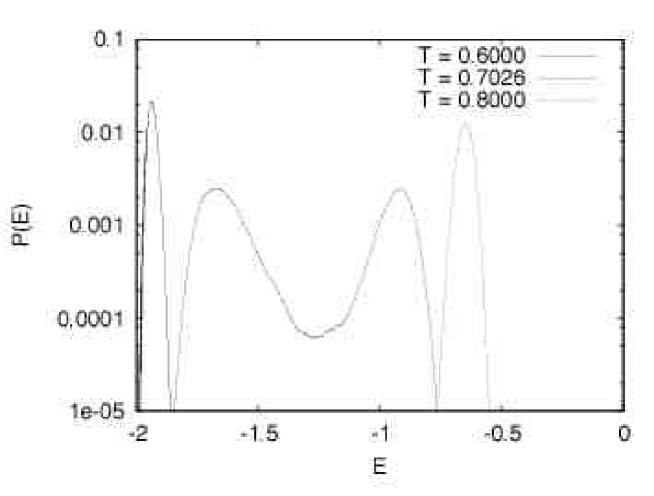
Figure 1: Probability distributions of energy of 2-dimensional 10-state Potts model at three temperatures: $T=0.6000$, 0.7026, and 0.8000. The results were obtained from a multicanonical MC simulation.

3 RESULTS

We now present the results of our simulations based on the algorithms described in the previous section.

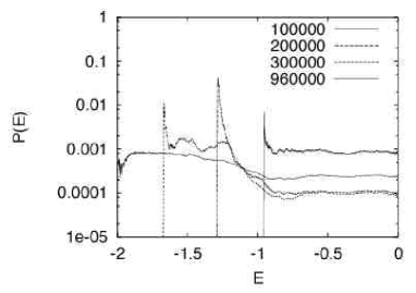
Figure 2: Iterative process of multicanonical weight factor determination for the 2-dimensional 10-state Potts model. The results after 100,000 MC sweeps, 200,000 MC sweeps, 300,000 MC sweeps, and 960,000 MC sweeps are superimposed.

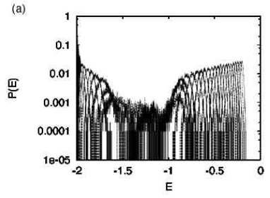
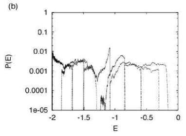
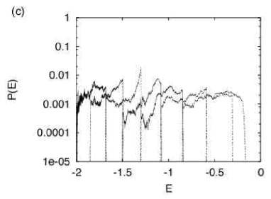
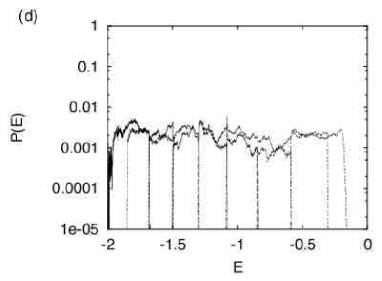
Figure 3: Probability distributions of energy for the 2-dimensional 10-state Potts model: the results of REM simulation with 32 replicas (a) and iterations of MUCAREM simulations with 8 replicas (b), (c), and (d).

The first example is a spin system. We studied the 2-dimensional 10-state Potts model [24]. The lattice size was $34\times 34$. This system exhibits a first-order phase transition [25]. In Figure 1 we show the probability distributions of energy at three tempeartures (above the critical temperature $T_{C}$, at $T_{C}$, and below $T_{C}$). At the critical temperature we observe two peaks in the distribution, indicating that the system indeed undergoes a first-order phase transition.

In Figure 2 we show how the iterative procedure [13] for the MUCA weight factor determination converges. We see that a flat distribution in the entire energy range was obtained after 960,000 MC sweeps. Note that the convergence slows down drastically near the global-minimum-energy region (step from 300,000 MC sweeps to 960,000 MC sweeps).

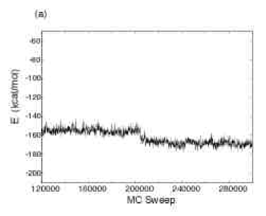
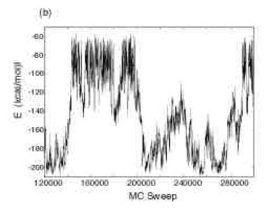
Figure 4: Time series (from 120,000 MC sweeps to 300,000 MC sweeps) of potential energy of the peptide fragment of ribonuclease T1 from a conventional canonical MC simulation at $T=200$ K (a) and a multicanonical MC simulation (b).

In Figure 3 we show the results of our new method for the MUCA weight factor determination. We first made a REM simulation of 10,000 MC sweeps (for each replica) with 32 replicas (Figure 3(a)). Using the obtained energy distributions, we determined the (preliminary) MUCA weight factor by the REMUCA procedure as described in the previous section. Because the trials of replica exchange are not accepted near the critical temperature for first-order phase transitions, the probability distributions in Figure 3(a) for the energy range from $\sim-1.5$ to $\sim-1.0$ fails to have sufficient overlap, which is required for successful application of REM. This means that the MUCA weight factor, or density of states, in this energy range thus determined is of “poor quality.” With this MUCA weight factor, however, we made iterations of three MUCAREM simulations of 10,000 MC sweeps (for each replica) with 8 replicas (Figures 3(b), 3(c), 3(d)). In Figure 3(b) we see that the distributions are not completely flat, reflecting the poor quality in the phase-transition region. This problem is rapidly rectified as iterations continue, and the distributions are completely flat in Figure 3(d), which gives an optimal MUCA weight factor in the entire energy range. The details including the comparisons with the new method in Ref. [14] will be published elsewhere [24].

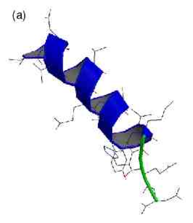
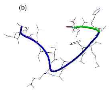
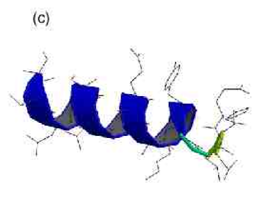
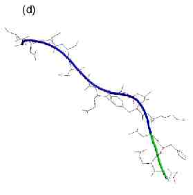
Figure 5: Typical snapshots from the multicanonical MC simulation of Figure 4(b). The corresponding numbers of MC sweeps are 138,000 (a), 190,000 (b), 243,000 (c), and 295,000 (d). The figures were created with Molscript and Raster3D.

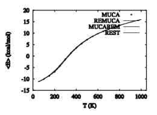
Figure 6: The average potential energy of Met-enkephalin in gas phase as a function of temperature. The results from the four generalized-ensemble algorithms, MUCA, REMUCA, MUCAREM, and REST, are superimposed.

The second example is a protein system. We first illustrate how effectively generalized-ensemble simulations can sample the configurational space compared to the conventional simulations in the canonical ensemble. It is known by experiments that the system of a 17-residue peptide fragment from ribonuclease T1 tends to form $\alpha$-helical conformations. We have performed both a canonical MC simulation of this peptide at a low temperature ($T=200$ K) and a multicanonical MC simulation [26]. In Figure 4 we show the time series of potential energy from these simulations.

We see that the canonical simulation thermalizes very slowly. On the other hand, the MUCA simulation indeed performs a random walk in potential energy space covering a very wide energy range. Four conformations chosen during this period (from 120,000 MC sweeps to 300,000 MC sweeps) are shown in Figure 5 for the MUCA simulation. The MUCA simulation indeed samples a wide conformational space.

The last example is a penta peptide, Met-enkephalin, whose amino-acid sequence is: Tyr-Gly-Gly-Phe-Met. In Figure 6, we show the average potential energy of Met-enkephalin in gas phase as a function of temperature that was calculated by the single- and multiple-histogram reweighting techniques from the four generalized-ensemble algorithms, MUCA, REMUCA, MUCAREM, and REST [27]. The results are in good agreement.

4 CONCLUSIONS

In this article we have described the formulations of the three well-known generalized-ensemble algorithms, namely, multicanonical algorithm (MUCA), simulated tempering (ST), and replica-exchange method (REM). We then introduced three new generalized-ensemble algorithms that combine the merits of the above three methods, which we refer to as replica-exchange multicanonical algorithm (REMUCA), replica-exchange simulated tempering (REST), and multicanonical replica-exchange method (MUCAREM).

With these new methods available, we believe that we now have working simulation algorithms for spin systems and protein systems.

5 Acknowledgements

Our simulations were performed on the HITACHI and other computers at the Research Center for Computational Science, Okazaki National Research Institutes. This work is supported, in part, by a grant from the Research for the Future Program of the Japan Society for the Promotion of Science (JSPS-RFTF98P01101).

References

- [1] U.H.E. Hansmann, Y. Okamoto, Y. Curr. Opin. Struct. Biol. 9 (1999) 177.
- [2] A.M. Ferrenberg, R.H. Swendsen, Phys. Rev. Lett. 61 (1988) 2635; ibid. 63 (1989) 1658.
- [3] A.M. Ferrenberg, R.H. Swendsen, Phys. Rev. Lett. 63 (1989) 1195; S. Kumar, D. Bouzida, R.H. Swendsen, P.A. Kollman, J.M. Rosenberg, J. Comput. Chem. 13 (1992) 1011.
- [4] B.A. Berg, T. Neuhaus, Phys. Lett. B267 (1991) 249; Phys. Rev. Lett. 68 (1992) 9.
- [5] B.A. Berg, Fields Institute Communications 26 (2000) 1; cond-mat/9909236.
- [6] U.H.E. Hansmann, Y. Okamoto, J. Comput. Chem. 14 (1993) 1333.
- [7] U.H.E. Hansmann, Y. Okamoto, in Annual Reviews of Computational Physics VI, D. Stauffer (Ed.) (World Scientific, Singapore, 1999) p. 129.
- [8] A.P. Lyubartsev, A.A. Martinovski, S.V. Shevkunov, P.N. Vorontsov-Velyaminov, J. Chem. Phys. 96 (1992) 1776; E. Marinari, G. Parisi, Europhys. Lett. 19 (1992) 451.
- [9] E. Marinari, G. Parisi, J.J. Ruiz-Lorenzo, in Spin Glasses and Random Fields, A.P. Young (Ed.) (World Scientific, Singapore, 1998) p. 59.
- [10] A. Irbäck, F. Potthast, J. Chem. Phys. 103 (1995) 10298.
- [11] U.H.E. Hansmann, Y. Okamoto, J. Comput. Chem. 18 (1997) 920.
- [12] G.R. Smith, A.D. Bruce, Phys. Rev. E 53 (1996) 6530.
- [13] B.A. Berg, Nucl. Phys. B (Proc. Suppl.) 63A-C (1998) 982.
- [14] F. Wang, D.P. Landau, Phys. Rev. Lett. 86 (2001) 2050.
- [15] K. Hukushima, K. Nemoto, J. Phys. Soc. Jpn. 65 (1996) 1604; K. Hukushima, H. Takayama, K. Nemoto, Int. J. Mod. Phys. C 7 (1996) 337.
- [16] M.C. Tesi, E.J.J. van Rensburg, E. Orlandini, S.G. Whittington, J. Stat. Phys. 82 (1996) 155.
- [17] A. Mitsutake, Y. Sugita, Y. Okamoto, Biopolymers (Peptide Science) 60 (2001) 96.
- [18] Y. Iba, Int. J. Mod. Phys. C 12 (2001) 623.
- [19] U.H.E. Hansmann, Chem. Phys. Lett. 281 (1997) 140.
- [20] Y. Sugita, Y. Okamoto, Chem. Phys. Lett. 314 (1999) 141.
- [21] Y. Sugita, A. Kitao, Y. Okamoto, J. Chem. Phys. 113 (2000) 6042.
- [22] Y. Sugita, Y. Okamoto, Chem. Phys. Lett. 329 (2000) 261.
- [23] A. Mitsutake, Y. Okamoto, Chem. Phys. Lett. 332 (2000) 131.
- [24] T. Nagasima, Y. Sugita, A. Mitsutake, Y. Okamoto, in preparation.
- [25] R.J. Baxter, J. Phys. C 6 (1973) L445.
- [26] A. Mitsutake, Y. Okamoto, in preparation.
- [27] A. Mitsutake, Y. Sugita, Y. Okamoto, in preparation.