The Kondo lattice model from strong-coupling viewpoint

Abstract

We study the magnetic excitation spectrum of the two-dimensional (2D) square-lattice S=1/2 Kondo lattice model at finite (hole) doping, by representing the Hamiltonian in terms of a set of local excitations. The location of the paramagnetic-antiferromagnetic phase boundary at T=0 is determined.

The Kondo lattice model in its simplest form describes itinerant ($c$) electrons hopping on a lattice, and interacting with localized ($d$) orbitals via Kondo exchange $J$ (we assume an antiferromagnetic sign $J\geq 0$):

$$H=-t\sum_{i,j,\sigma}\left(c_{\sigma,i}^{\dagger}c_{\sigma,j}+\mbox{h.c.}\right)+J\sum_{i}{\bf S}_{i}^{d}.{\bf S}_{i}^{c}.$$ (1)

There are two major issues that are of interest from both fundamental and experimental (heavy fermion materials) perspectives: (1.) Description of the competition between the Kondo effect and the RKKY interaction, which generally leads to a quantum phase transition from a paramagnetic to a long-range ordered phase, and (2.) The possible breakdown of the Kondo effect (screening) near such a phase boundary, especially in antiferromagnetic metals [1]. We concentrate mostly on the first aspect, and consider the model Eq.(1) on a square lattice at finite hole doping $\delta$ ($\delta=0$ is half-filling), which makes the system conducting.

We rewrite Eq.(1) in the local (one site) basis, where four bosonic modes (a singlet and a triplet) can be excited: $\sqrt{2}s^{\dagger}|v\rangle=\epsilon_{\sigma\rho}c_{\sigma}^{\dagger}d_{\rho}^{\dagger}|0\rangle$, $\sqrt{2}t_{\alpha}^{\dagger}|v\rangle=\sigma_{\rho\delta}^{\alpha}\epsilon_{\delta\sigma}c_{\sigma}^{\dagger}d_{\rho}^{\dagger}|0\rangle$, $(\alpha=x,y,z;\ \sigma,\rho,\delta=\uparrow,\downarrow)$, as well as two fermionic modes: $f_{1,\sigma}^{\dagger}|v\rangle=d_{\sigma}^{\dagger}|0\rangle$, $f_{2,\sigma}^{\dagger}|v\rangle=c_{\uparrow}^{\dagger}c_{\downarrow}^{\dagger}d_{\sigma}^{\dagger}|0\rangle$. Here $|v\rangle$ is a reference vacuum with no excitations present, and $|0\rangle$ corresponds to absence of physical electrons. The described set of states can be used to generalize the bond-operator representation, often used in localized spin systems (with only $s$ and ${\bf t}$ modes present) [2]. Similar ideas have also been successfully applied to Kondo insulators ($\delta=0$) [3]. The representation is exact provided the on-site kinematic constraint is implemented: $s^{\dagger}s+f_{\nu,\sigma}^{\dagger}f_{\nu,\sigma}+t_{\alpha}^{\dagger}t_{\alpha}=1$, necessary to restrict the Hilbert space of the new operators to the physical sub-space. It is physically clear that for doping $\delta=0$ and strong Kondo exchange $J/t\gg 1$ the ground state is a singlet (thus paramagnet), meaning that the $s$ excitations condense: $\langle s\rangle\neq 0$. Let us note that the term “strong-coupling” ($J/t\gg 1$) in this work has the opposite meaning to the one used in Ref.[1]. The Hamiltonian in the local representation becomes, by taking the singlet state $s^{\dagger}|v\rangle$ as the ground state, $H=H_{2}+H_{Int}$:

$$\!\!H_{2}\!=\!\!\!\sum_{{\bf k},\sigma,\nu=1,2}E_{\nu}({\bf k})f_{\nu,\sigma,{\bf k}}^{\dagger}f_{\nu,\sigma,{\bf k}}+J\sum_{{\bf k}}{\bf t}_{{\bf k}}^{\dagger}.{\bf t}_{{\bf k}}+\sum_{{\bf k},\sigma}B({\bf k})f_{1,\sigma,{\bf k}}^{\dagger}f_{2,-\sigma,-{\bf k}}^{\dagger}+\mbox{h.c.},$$ (2)

$$H_{Int}=\ \sum\ [{\bf t}{\bf t}ff]\ \&\ [{\bf t}ff]\ \mbox{scattering}\ \mbox{vertices},$$ (3)

where $E_{\nu}({\bf k}),B({\bf k})\propto t$ are easily calculated, and $H_{Int}$ represents the non-linear interactions (with coefficients also proportional to the hopping $t$) between the bosonic and fermionic modes. The challenge now becomes to treat the kinematic constraint (which amounts to an infinite local repulsion between the ${\bf t}$ and $f_{\nu}$ modes), as well as the interactions present in $H_{Int}$, as accurately as possible in order to have reliable results for the excitation spectrum. We have followed the philosophy outlined in Ref.[4] for spin insulators to implement the hard-core repulsion, while the various terms in $H_{Int}$ were treated to lowest non-trivial (one-loop) order (see also references [5] and [6], discussing the situation at finite doping for the $t-J$ model). The extension of the approach from zero to finite doping is a non-trivial matter, and details will be provided elsewhere [7]. It is crucial in this treatment that the S=1 magnetic excitations (the spectrum of the ${\bf t}$ operators) form a dilute Bose gas. Departure from the dilute, low-density limit would also mean a possible change in the ground state and failure of our approximation scheme since the latter is based on classification of diagrams in powers of the excitation density. In addition, doping is also assumed to be a small parameter in the problem.

Let us summarize our main results [7]:
$\bullet$ The magnetic (${\bf t}$) excitations are found to be gapped everywhere in a certain region of parameter space, see Fig.1, meaning that the system is paramagnetic. The gap at the antiferromagnetic ordering wave vector ${\bf Q}_{AF}=(\pi,\pi)$ vanishes on a critical line, signaling a transition to a phase with long-range order (finite staggered magnetization, proportional to the condensate $\langle{\bf t}_{{\bf k}={\bf Q}_{AF}}\rangle$). The parameter F, displayed on the axis in Fig.1 (which is introduced for numerical reasons), is found to vary very weakly with doping. In the simplest of our approximation schemes it has the constant value F$\approx 0.72$ [7]. This produces a critical point at zero doping $(J/t)_{c}\approx 1.39$ which is quite close to the numerical result [8] (however no numerical results are available for $\delta\neq 0$). Let us also mention that the magnons are damped at any finite doping, which can readily be seen from the width of their spectral function.
$\bullet$ We would like to emphasize that our calculational scheme is self-consistent in the sense that the dilute Bose gas description is maintained throughout the phase diagram. This means that the singlet ground state, the starting point of the calculation, is stable (i.e. $\langle s\rangle\neq 0$), leading to the usual Fermi liquid description of the critical properties [9]. Departure from the Fermi liquid picture would occur if $\langle s\rangle\rightarrow 0$ at the quantum critical point (QCP); one can then expect various exotic effects such as different critical exponents, which has been in fact suggested to occur in two dimensions [1]. The fact that we do not find perturbative indications for breakdown of the Kondo effect at the QCP could be quite possibly due to our approximation scheme, which can detect the existence of a quantum critical line (where [the magnetic gap]$\ll J$), but is not capable of predicting universal properties in the quantum critical regime.

We gratefully acknowledge stimulating conversations with Kevin Ingersent and Subir Sachdev, and the financial support of NSF Grant DMR-9974396.

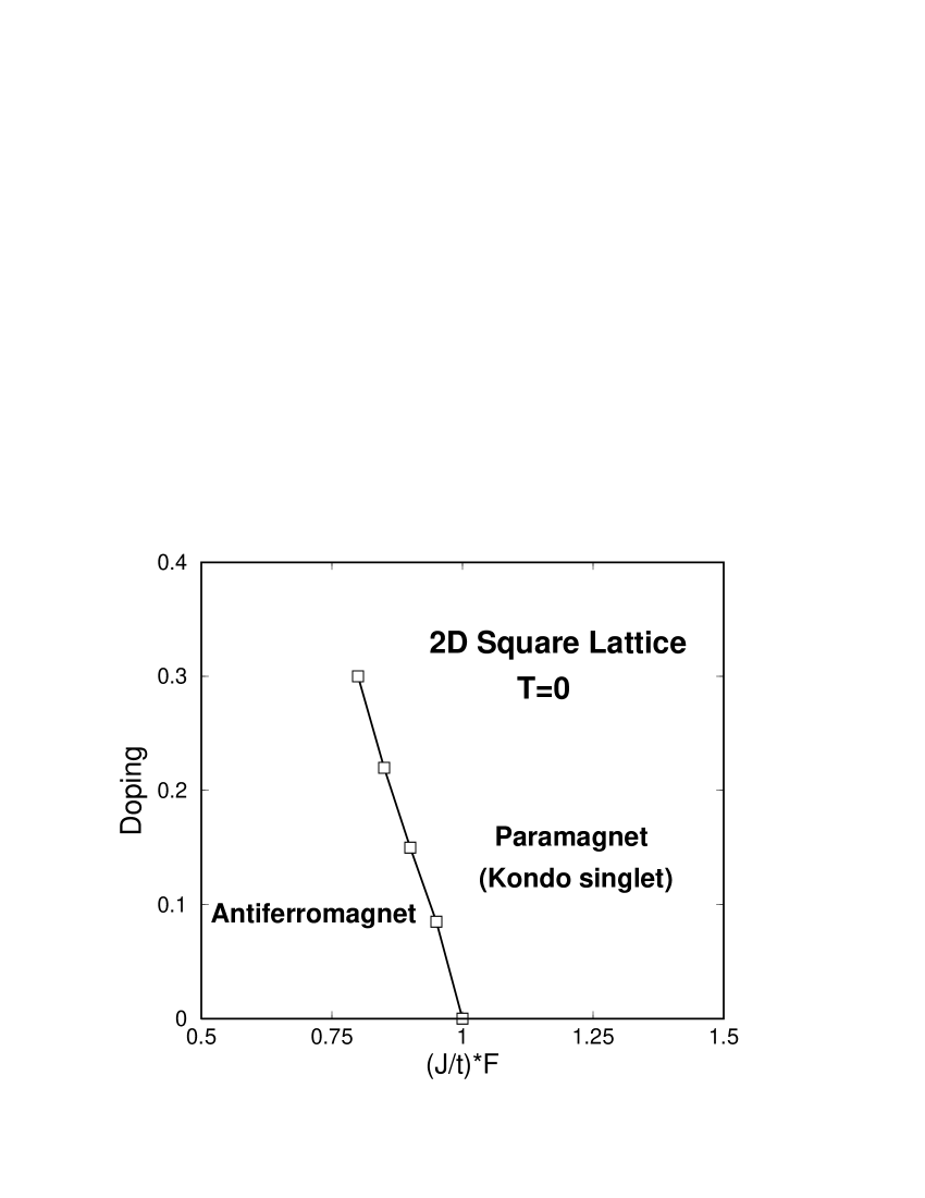
Figure 1: Phase diagram of the Kondo lattice model.

References

- [1] P. Coleman, C. Pepin, Q. Si, and R. Ramazashvili, J. Phys. Cond. Matt. 13 (2001) 723; Q. Si, S. Rabello, K. Ingersent, and L. Smith, Nature 413 (2001) 804; P. Coleman, Physica B 259-261 (1999) 353, and references therein.
- [2] S. Sachdev and R.N. Bhatt, Phys. Rev. B 41 (1990) 9323.
- [3] C. Jurecka and W. Brenig, Phys. Rev. B 64 (2001) 092406; R. Eder, O. Rogojanu, and G.A. Sawatzky, Phys. Rev. B 58 (1998) 7599; M. Kato and T. Tsuneto, Prog. Theor. Phys. 74 (1985) 670.
- [4] V.N. Kotov, O. Sushkov, W.H. Zheng, and J. Oitmaa, Phys. Rev. Lett. 80 (1998) 5790, and cited references.
- [5] O.P. Sushkov, Phys. Rev. B 63 (2001) 174429.
- [6] K. Park and S. Sachdev, Phys. Rev. B 64 (2001) 184510.
- [7] V.N. Kotov and P.J. Hirschfeld, in preparation.
- [8] S. Capponi and F.F. Assaad, Phys. Rev. B 63 (2001) 155114; F.F. Assaad, Phys. Rev. Lett. 83 (1999) 796, and cited references.
- [9] J. Hertz, Phys. Rev. B 14 (1976) 1165; A.J. Millis, Phys. Rev. B 48 (1993) 7183.