On the non-orthogonality problem in the description of quantum devices

Abstract

An approach which allows to include the corrections from non-orthogonality of electron states in contacts and quantum dots is developed. Comparison of the energy levels and charge distributions of electrons in 1D quantum dot (QD) in equilibrium, obtained within orthogonal (OR) and non-orthogonal representations (NOR), with the exact ones shows that the NOR provides a considerable improvement, for levels below the top of barrier. The approach is extended to non-equilibrium states. A derivation of the tunneling current through a single potential barrier is performed using equations of motion for correlation functions. A formula for transient current derived by means of the diagram technique for Hubbard operators is given for the problem of QD with strongly correlated electrons interacting with electrons in contacts. The non-orthogonality renormalizes the tunneling matrix elements and spectral weights of Green functions (GFs).

Keywords: non-orthogonality, current, tunneling
Poster, your reference: MoP-06

Introduction: In the description of tunneling processes through quantum devices two approaches are useful: 1) the wave functions used for calculation of the Green functions fulfil the boundary conditions for the whole device, or 2) a subdivision of the system is made [1, 2, 3, 4, 5, 6] and then the wave functions corresponding to different subsystems are, in general, not orthogonal to each other. The second approach is preferable if the strength of the interactions in different regions of the system differ considerably. In this framework tunneling arises due to the non-orthogonality of the wave functions from different subsystems. Prange [1] found in his investigation of SNS- and SIS-junctions, that an overcomplete non-orthogonal basis set, allowing for the desirable separation leads to corrections from overlap integrals of the same order as the tunneling coefficients. Hence, it is essential to take the overlap between the orbitals into account. We also note the conclusion of Svidzinskii [7], that the tunneling Hamiltonian approach is useful only if one is interested in linear responses.

We present results of a different approach based on the diagram technique for Hubbard operators within non-orthogonal basis [8]. Generalized to non-equilibrium states, the method still allows for calculations in the language of model subsystems.

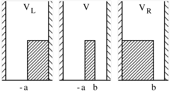
Figure 1: Fransson et al.

Equilibrium: Consider a finite box with hard walls containing a barrier of finite height $V_{0}$ see Fig. 1; the Hamiltonian is ${\cal H}=\frac{p^{2}}{2m}+V$. We approximate this system by two separate subsystems for which $\{\phi_{p},\varepsilon_{p}\}$ and $\{\phi_{q},\varepsilon_{q}\}$ are complete ON eigensystems of the ‘left’ (L) and ‘right’ (R) Hamiltonians ${\cal H}_{L}=\frac{p^{2}}{2m}+V_{L}$, $p\in L$ and ${\cal H}_{R}=\frac{q^{2}}{2m}+V_{R}$, $q\in R$ corresponding to the potentials $V_{L}=V\Theta(-x+b)+(V_{0}+V)\Theta(x-b)$ and $V_{R}=(V_{0}+V)\Theta(-x-a)+V\Theta(x+a)$ see Fig 1; $\Theta(x)$ is the Heaviside step function. Introduce the field operators $\psi_{L}(x)=\sum_{p\sigma}a_{p\sigma}\phi_{p}(x)$ and $\psi_{R}(x)=\sum_{q\sigma}a_{q\sigma}\phi_{q}(x)$; $\sigma$ denotes spin. The exact field operator is expanded as $\psi=\psi_{A}+\psi_{B}$ where $\psi_{A}=\psi_{L}+\psi_{R}$ and $\psi_{B}$ is a reminder. Assuming $\psi_{B}=0$ yields the approximate Hamiltonian ${\cal H}_{A}=\sum_{k\sigma}\varepsilon_{k}a_{k\sigma}^{\dagger}a_{k\sigma}+\sum_{pq\sigma}\left(t_{pq}a_{p\sigma}^{\dagger}a_{q\sigma}+H.c.\right)$ ,where $t_{kk^{\prime}}=\int\phi_{k}^{*}\left(\frac{p^{2}}{2m}+V\right)\phi_{k^{\prime}}{\rm d}x$; $k=p,q$. Then $t_{pq}={\cal O}_{{p}{q}}\varepsilon_{q}+W_{pq}$, where ${\cal O}_{{p}{q}}\equiv\int\phi_{p}^{*}\phi_{q}{\rm d}x$ defines the overlap matrix and $W_{pq}\equiv\int\phi_{p}^{*}(V-V_{R})\phi_{q}{\rm d}x$, and similarly for the other matrix elements. Neglect the differences $W_{kk^{\prime}}$ whenever $k,k^{\prime}$ belong to the same contact. The operators $a_{p\sigma}$ are defined by $a_{p\sigma}=\sum_{p^{\prime}}{\cal O}^{-1}_{{p}{p^{\prime}}}\int\phi_{p^{\prime}}^{*}(x)\psi(x){\rm d}x+\sum_{q^{\prime}}{\cal O}^{-1}_{{p}{q^{\prime}}}\int\phi_{q^{\prime}}^{*}(x)\psi(x){\rm d}x$, and similarly for $a_{q\sigma}$. Then, the anti-commutation relations are $\{{a_{k\sigma}},{a_{k^{\prime}\sigma}^{\dagger}}\}={\cal O}^{-1}_{{k}{k^{\prime}}}$, where ${\cal O}^{-1}_{{k}{k^{\prime}}}$ is element $kk^{\prime}$ of the inversed overlap matrix. Solutions of the Dyson equation $g_{A}^{-1}=g_{0}^{-1}-{\cal O}^{-1}W$ for ${\cal O}^{-1}=I$ (OR), $I$ is the identity operator, ${\cal O}^{-1}\neq I$ (NOR) compared to the exact solution are shown in Table 1. As seen, the improvement achieved in NOR is considerable. However, in the proximity of the barrier height corrections from the reminder $\psi_{B}$ should be taken into account when calculating the charge distribution, even though the energy levels estimated by NOR still are much better.

Transient current: Transient current can be calculated [2] from $-e\frac{d}{dt}\langle{N_{L}}\rangle$, where $N_{L}$ is the number of carriers in the cylinder with top and bottom areas $S$ and axis parallel to current. The tunneling matrix elements now contain the vector potential, so, in the Hamiltonian ${\cal H}_{A}$ substitute $t_{kk^{\prime}}$ by $T_{kk^{\prime}}=\langle k|({\bf k}-(e/c){\bf A}(t))^{2}+V|k^{\prime}\rangle$, the non-equilibrium tunneling coefficients. Whenever $k,k^{\prime}$ belong to the same contact we approximate $T_{kk^{\prime}}$ by its corresponding equilibrium value and neglect the differences $W_{kk^{\prime}}$, yielding for example $T_{pp^{\prime}}\rightarrow\varepsilon_{p}$.

Via the transformation $a_{p(q)\sigma}=e^{-i\varphi_{L(R)}(t)}l_{p\sigma}(r_{q\sigma})$, which allows to introduce current states, we derive a tunneling current $J\sim|T|^{2}$ as a function of the applied voltage $eV=\mu_{L}-\mu_{R}\approx\frac{\varphi(t)-\varphi(t^{\prime})}{t-t^{\prime}}$, where the phase $\varphi=\varphi_{L}-\varphi_{R}$. Putting ${\cal O}^{-1}_{{k}{k^{\prime}}}=\delta_{kk^{\prime}}$ when $k,k^{\prime}$ belong to the same contact, is consistent with the approximation. Note that with this assumption $\langle{N_{L}}\rangle=\sum_{p\sigma}{\cal S}_{{p}{}}\langle{n_{p\sigma}}\rangle$, where $n_{p\sigma}=a_{p\sigma}^{\dagger}a_{p\sigma}$ and ${\cal S}_{{p}{}}={\cal S}_{{p}{p}}$ is a part of the overlap matrix, obtained by integration over the volume in which $-e\frac{d}{dt}\langle\hat{N}_{L}\rangle$ is calculated. The equations of motion for $\langle{n_{p\sigma}}\rangle$ is $\frac{{\rm d}}{{\rm d}t}\langle{n_{p\sigma}}\rangle=2{\rm Im}\sum_{q}\tilde{T}_{pq}e^{i\varphi(t)}\langle{l_{p\sigma}^{\dagger}r_{q\sigma}}\rangle$ where $\langle{l_{p\sigma}^{\dagger}r_{q\sigma}}\rangle=\tilde{T}_{pq}(f_{p}-f_{q})\frac{(-i)^{2}}{\Delta_{qp}+eV-i\delta}$, $\Delta_{qp}=\varepsilon_{q}-\varepsilon_{p}$, $\tilde{T}_{pq}=T_{pq}+{\cal O}^{-1}_{{p}{q}}\varepsilon_{q}$ in the given approximation and $f$ is the Fermi function. The resulting current formula in terms of densities of states $N_{L}(\mu)$ and $N_{R}(\mu)$ then is $J=V\cdot 4\pi e^{2}S{\cal S}|\tilde{T}|^{2}N_{L}(\mu)N_{R}(\mu)\equiv VR^{-1},$ (the factor 2 is due to spin). Thus, in this approximation the only change required is replacing $T\rightarrow\tilde{T}$.

Strong correlations in quantum dot: Physically, the coupling arises due to overlap of wave functions. When the system is close to the regime of Coulomb blockade, the overlap is small and the interaction between subsystems is much weaker than the one inside the QD, i.e. the matrix element of tunneling $|T|<<\Delta_{\bar{a}}=E_{\Gamma_{n+1}}-E_{\Gamma_{n}}$; here $E_{\Gamma_{n}}$ is an eigenvalue of the Hamiltonian of the QD, $H_{d}|\Gamma\rangle=E_{\Gamma}|\Gamma\rangle$; $a=[\Gamma_{n},\Gamma_{n+1}]$ is a fermion-like transition ($\bar{a}=[\Gamma_{n+1},\Gamma_{n}]$) which is described by Hubbard operator $X^{\Gamma_{n}\Gamma_{n+1}}\equiv X^{a}$. In this situation the states of the QD will be perturbed only slightly, therefore QD should be described by many-electron states. Here we will demonstrate how the technique developed in ref. [8] for correlated electron systems for thermodynamics can be extended to non-equilibrium phenomena. Since the Hamiltonian includes strong Coulomb interactions inside QD, the terms of the kind $v_{k\sigma,\mu_{2}\mu_{3}\mu_{4}}l_{k\sigma}^{\dagger}d_{\mu_{2}}^{\dagger}d_{\mu_{3}}d_{\mu_{4}}=v_{k\sigma,\mu_{2}\mu_{3}\mu_{4}}(d_{\mu_{2}}^{\dagger}d_{\mu_{3}}d_{\mu_{4}})^{a}l_{k\sigma}^{\dagger}X^{a}\equiv T_{k\sigma,a}^{Coul}l_{k\sigma}^{\dagger}X^{a}$, also contribute to the process of electron tunneling from the left contact to the QD and should not be decoupled in Hartree-Fock fashion. We include these interactions to the Hamiltonian of coupling (see ref. [8]). The total Hamiltonian then is:

$${\cal H}=\sum_{k\sigma}\varepsilon_{k\sigma}c_{k\sigma}^{\dagger}c_{k\sigma}+\sum_{\Gamma}E_{\Gamma}X^{\Gamma\Gamma}+\sum_{k\sigma,a}(T_{k\sigma,a}c_{k\sigma}^{\dagger}X^{a}+H.c.)$$

where $k=p,q$ ($p\in L$ and $q\in R$). Any $X$-operator can be rewritten in terms of products of single-electron operators $d,d^{\dagger}$ of QD and, therefore, using $\{c_{k\sigma},d_{\mu}^{\dagger}\}={\cal O}_{k\sigma}^{-1}{}_{,\mu}$ one can show [8] that $\{c_{k\sigma},X^{\bar{a}}\}={\cal O}_{k\sigma}^{-1}{}_{,\mu}(d_{\mu})^{b}\varepsilon_{\xi}^{b\bar{a}}X^{\xi}$, where $\xi$ is a Bose-like transition, and $\varepsilon_{\xi}^{b\bar{a}}$ defines commutation relations between $X$-operators in the uncoupled system, $\{X^{b},X^{\bar{a}}\}=\varepsilon_{\xi}^{b\bar{a}}X^{\xi}.$ Strictly speaking, when the coupling is switched on, the many-electron states also become non-orthogonal to each other but the corrections contain higher order products of ${\cal O}^{-1}_{{k\sigma,}{\mu}}$. Hence, we neglect these corrections since we are only interested in first order with respect to transparancy. Following ref. [2] we calculate the contribution to the current from ‘left’ electrons $J_{tr}^{(l)}=-2eS{\cal S}{\rm Re}\sum_{k\sigma,a}\tilde{T}_{k\sigma,a}^{(l)*}G_{k\sigma,\bar{a}}^{<}(tt)$, where $\tilde{T}_{k\sigma,a}^{(l)}=T_{k\sigma,a}+{\cal O}^{-1}_{{k\sigma,}{\mu}}(d_{\mu})^{b}\varepsilon_{a}^{b\Gamma}E_{\Gamma}$. The additional term comes from the anti-commutation of $c_{k\sigma}$ and the QD Hamiltonian ${\cal H}_{D}$. Expressing the current in terms of retarded and ‘lesser’ GFs of the QD, $G_{a\bar{a}}^{R}$ and $G_{a\bar{a}}^{<}$ respectively, yields:

$$J_{tr}^{(l)}=2eS{\cal S}{\rm Im}\sum_{k\sigma,a}\left\{\tilde{T}_{k\sigma,a}^{(l)*}{\cal O}^{-1}_{{k\sigma}{,\mu}}(d_{\mu})^{a}P^{a}f_{L}(\varepsilon_{k\sigma})-|\tilde{T}_{k\sigma,a}^{(l)}|^{2}[G_{a,\bar{a}}^{<}(\varepsilon_{k\sigma})+f_{L}(\varepsilon_{k\sigma})G_{a,\bar{a}}^{R}(\omega)_{|\varepsilon_{k\sigma}}]\right\}$$

For a transition $a=[\gamma,\Gamma]$ the expectation value $P^{a}=\langle{\{{X^{\gamma\Gamma}},{X^{\Gamma\gamma}}\}}\rangle=N^{\gamma}+N^{\Gamma}$, i.e. it is a sum of the population numbers corresponding to the transition. They should be found from $\int G_{a,\bar{a}}^{<(>)}(\omega)d\omega$. The system for $G_{a,\bar{a}}^{<(>)}(\omega)$ is very cumbersome and therefore not given here. However, physics is seen from the form of the retarded GF: $G_{a,\bar{a}}^{R}(\omega)=\frac{[1+\gamma(\omega)]P^{a}}{\omega+i\delta-\Delta_{\bar{a}}-\Gamma_{a}(\omega)P^{a}},$ where $\Gamma_{a}(\omega)=\Gamma_{a}^{(l)}(\omega)+\Gamma_{a}^{(r)}(\omega)$, $\gamma_{a}(\omega)=\gamma_{a}^{(l)}(\omega)+\gamma_{a}^{(r)}(\omega)$, and the width $\Gamma_{a}^{(l)}(\omega)=\sum\tilde{T}_{p\sigma,a}^{(l)*}g_{p\sigma}(\omega)\tilde{T}_{p\sigma,a}^{(l)}$. $g$ is bare GF of ‘left’ electrons, $\gamma_{a}^{(l)}(\omega)=\tilde{T}_{p\sigma,a}^{(l)*}g_{p\sigma}(\omega){\cal O}^{-1}_{{p\sigma,}{\mu}}(d_{\mu})^{b}P^{b}$ and in $\Gamma_{a}^{(r)}(\omega)$, $\gamma_{a}^{(r)}(\omega)$ summation is over $q,\sigma$. Thus, each single-electron intra-dot transition acquires width, which depends on the overlap of the wave function of conduction electron in the left(right) contact with energy near Fermi level $\mu_{L}(\mu_{R})$ with those in-dot orbitals in transition $a$.

In conclusion we have shown that, the separation of a device into auxiliary subsystems unavoidably leads to eigenbases non-ortogonal to one another. This results in additional contributions to matrix elements of tunneling and in redistribution of spectral weights since part of charge is in ‘intermediate’ state. Precision of calculations is improved even in the most ‘dangerous’ region at the top of the barrier.

Exact	OR	NOR
0.28	0.012	0.29
1.06	0.80	1.08
2.28	2.07	2.30
4.04	3.31	4.18

Table 1: Energy levels (mHartree) for barrier width 1 Bohr and height 4.1 mHartree.

Caption

• The assumed potentials - ‘left’, ‘exact’ and ‘right’.

References

• [1] R.E. Prange, Phys Rev Lett 131, 1083 (1963).
• [2] Y. Meir and N.S. Wingreen, Phys Rev Lett 68, 2512 (1992).
• [3] Y. Kuramoto, H. Sakaki, T. Inoshita and A. Shimizu, Phys Rev B 48, 14725 (1993).
• [4] A.P. Jauho, N.S. Wingreen and Y. Meir, Phys Rev B 50, 5528 (1994).
• [5] A. Oguri and H. Ishii, Phys Rev B 51, 4715 (1995).
• [6] H. Sakaki, T. Inoshita and Y. Kuramoto, Superlatt. and Microstr. 22, 75 (1997).
• [7] A.V. Svidzinskii, Space-non-homogeneous problems in superconductivity (Nauka, Moscow, 1982) (in russian).
• [8] I.S. Sandalov, B. Johansson and O. Eriksson, to be published