Effects of non-orthogonality in the time-dependent current through tunnel junctions

Abstract

A theoretical technique which allows to include contributions from non-orthogonality of the electron states in the leads connected to a tunneling junction is derived. The theory is applied to a single barrier tunneling structure and a simple expression for the time-dependent tunneling current is derived showing explicit dependence of the overlap. The overlap proves to be necessary for a better quantitative description of the tunneling current, and our theory reproduces experimental results substantially better compared to standard approaches.
PACS numbers: 72.10.Bg, 72.15.-v, 73.23.-b, 73.40.Gk, 73.63.-bk

Achievements in nano-materials science is expected to have importance in many scientific fields, including information technology, quantum computing and fuel cells. In particular, tunneling phenomena have been under focus recently, both in magnetic heterostructures as well as for quantum dot systems. The purpose of this paper is to develop an improved description of this phenomenon for general tunnel junctions, with possible application to the aforementioned scientific questions.

To focus the discussion, we mention that conductance measurements on extremely small metal-insulator-metal (MIM) junctions were carried out by Vullers et al.[1] showing a non-linear conductance as a function of the bias voltage for low temperatures. The same behaviour has been reported for MIM double junctions[2] and Ti/TiO_x tunneling barrier systems[3, 4, 5]. The non-linearity in the current-voltage $(J-V)$ characteristics appears for source-drain bias voltages larger than the spacing of the quasi one dimensional subbands since different numbers of subbands become available for transport in the forward and reverse directions [6]. In the study by Simmons [7] the current was found to depend non-linearly on the voltage, roughly as $V+\gamma V^{3}$.

Many theoretical studies of transport in nanostructures with tunneling barriers rely on the transfer Hamiltonian[8, 9, 10, 11, 12] which contains serious inconsistencies [13]. The principle of the transfer Hamiltonian is a division of the system into subsystems. This is motivated by the fact that the physical properties of the subsystems may be different and, hence, require different descriptions. Another motivation is that one is directly offered the possibility to generalize the approach to any number of tunneling barriers in the system. The transfer (tunneling) between the subsystems arises due to an overlap of the wave functions in the region of the barrier whereas the electron operators of the different subsystems are assumed to be anti-commuting. Qualitatively this may be motivated since the leakage of a wave function in one subsystem into the other is exponentially small. The $J-V$ characteristics given in this picture also shows a non-linear structure for large bias voltages. Quantitatively, though, the assumption of anti-commuting operators creates serious errors in the calculations of the current. This becomes particularly evident in the equilibrium situation displayed in Table I, in which the four lowest states of a particle in a one dimensional hard walled box with a scattering potential are given. The energy levels are, as expected, reproduced within the non-orthogonal representation (NOR) with much higher accuracy than in the orthogonal representation (OR). Attempts that go beyond the transfer Hamiltonian have been made, e.g. by expanding the non-orthogonal states into a new Hilbert space [14]. However, the proven success and physical transparency of the transfer Hamiltonian approach makes it desirable to extend its applicability to more general situations where the overlap is large, without making use of perturbation theory. This can indeed be achieved, which we demonstrate in this paper.

In order to overcome the inconsistencies with the transfer Hamiltonian formalism, we develop a theoretical approach for time-dependent transport through tunneling systems in which the overlap between the subsystems give explicit contribution to the current. Technically, we will express the properties of the original system in terms of the operators constructed of the wave functions of each subsystem. The resulting model structurally resembles the transfer Hamiltonian, although the physical interpretation is different. We have chosen the single barrier system simply to show the features of our approach. The main result of this paper is the Eqn. (8) for the time-dependent tunneling current through a single barrier. This expression is applied to a MIM junction in order to analyze the effect of overlap on the current. To our knowledge there does not exist any derivation nor analysis of time-dependent transport in tunneling junctions where the non-orthogonality is not disregarded.

Let us now proceed starting with the one particle Hamiltonian

$\displaystyle H=\frac{p^{2}}{2}+V,$

where $V$ is any potential describing a system of two leads with an insulating layer in between. We introduce the two potentials $V_{\alpha},\ \alpha=L,R$, for the left $(L)$ and the right $(R)$ subsystem, respectively[8, 9, 15]. For instance, the left potential can be written as $V_{L}=V(x)\theta(-x+a_{L})+V(a_{L})\theta(x-a_{L})$, where $\theta(x)$ is the Heaviside function and $a_{L}$ is a turning point for the left subsystem. In each subsystem there are orthonormal eigenstates $\{\phi_{k},\varepsilon_{k\sigma}\}_{k\sigma\in\alpha}$ from which the corresponding field operator $\psi_{\alpha}(t,x)=\sum_{k\sigma\in\alpha}c_{k\sigma}(t)\phi_{k}(x)$ is constructed. Here $t$ is time and $x=({\bf r},\sigma)$ is a vector of the spatial coordinate ${\bf r}$ and the spin $\sigma$. Suppose that $\psi$ is the field operator of the system formed by the potential $V$. Then, this operator can be expanded in terms of $\psi_{\alpha}$ by the trivial identity $\psi(t,x)=\sum_{\alpha}\psi_{\alpha}(t,x)+[\psi(t,x)-\sum_{\alpha}\psi_{\alpha}(t,x)]$. Following reference[16] we project $\psi$ onto the subsystem $\alpha$ by

$\displaystyle\tilde{c}_{k\sigma}(t)=\int\phi_{k}^{*}(x)\psi(t,x){\rm d}x,$

$k\in\alpha$, interpreted as the annihilation of a particle in the state $\phi_{k}$ with spin projection $\sigma$. Creation $\tilde{c}^{\dagger}_{k\sigma}$ of a particle in the state $\phi_{k}$ is defined similarly. These projections are possible to use directly for a second quantized form of the Hamiltonian. However, such an expansion gives an inconvenient expression of the Hamiltonian with the overlap matrix appearing explicitly. Thus, in order to proceed further, we define the operators

$$\begin{array}[]{rcl}c_{k\sigma}(t)&=&\sum_{k^{\prime}}{\cal O}^{-1}_{{k}{k^{\prime}}}\tilde{c}_{k^{\prime}\sigma}(t),\\ c_{k\sigma}^{\dagger}(t)&=&\sum_{k^{\prime}}\left({\cal O}^{-1}_{{k}{k^{\prime}}}\right)^{*}\tilde{c}^{\dagger}_{k^{\prime}\sigma}(t),\end{array}$$ (1)

where $k^{\prime}$ runs over all states in $L\cup R$ and ${\cal O}^{-1}_{{k}{k^{\prime}}}$ is the element $kk^{\prime}$ of the inverse of the overlap matrix of the wave functions $\phi_{k},\ \phi_{k^{\prime}}$ given by ${\cal O}_{{k}{k^{\prime}}}=\mathop{\langle\phi_{k}|\phi_{k^{\prime}}\rangle}={\cal O}_{{k^{\prime}}{k}}^{*}$. By a limitation to the case of spin conservation we can omit the spin indices in the overlap integral. The expectation value of the Hamiltonian in these operators is

$${\cal H}=\int\psi^{\dagger}H\psi{\rm d}x={\cal H}_{L}+{\cal H}_{R}+{\cal H}_{T},$$ (2)

where we have defined ${\cal H}_{\alpha}=\int\psi_{\alpha}^{\dagger}H\psi_{\alpha}{\rm d}x$ and ${\cal H}_{T}=\sum_{\alpha\alpha^{\prime}}(\int\psi_{\alpha}^{\dagger}H\psi_{\alpha^{\prime}}{\rm d}x+H.c.)$. Here, we have neglected all expectation values that contain $\psi-\sum_{\alpha}\psi_{\alpha}$. Furthermore, we note that from the identity $V=V_{\alpha}+[V-V_{\alpha}],\ \alpha=L,R$, we find that the Hamiltonian of the lead ${\cal H}_{\alpha}=\sum_{k\sigma\in\alpha}\varepsilon_{k\sigma}c_{k\sigma}^{\dagger}c_{k\sigma}+\sum_{kk^{\prime}\in\alpha}\langle\phi_{k}|(V-V_{\alpha})|\phi_{k^{\prime}}\rangle c_{k\sigma}^{\dagger}c_{k^{\prime}\sigma},\ \alpha=L,R$. The last term is a sum of terms proportional to the integral of $\phi_{k}^{*}\phi_{k^{\prime}}$ over $(a_{R},\infty)$ or $(-\infty,a_{L})$ when $\alpha=L$ or $\alpha=R$, respectively, in which domains the wave functions are exponentially small. Thus, this term is negligible and we arrive at the appealing form of the Hamiltonian

$${\cal H}=\sum_{p\sigma\in L}\varepsilon_{p\sigma}c_{p\sigma}^{\dagger}c_{p\sigma}+\sum_{q\sigma\in R}\varepsilon_{q\sigma}c_{q\sigma}^{\dagger}c_{q\sigma}+\sum_{pq\sigma}(v_{pq\sigma}c_{p\sigma}^{\dagger}c_{q\sigma}+H.c.),$$ (3)

where $v_{pq\sigma}=\langle\phi_{p}|H|\phi_{q}\rangle$ is the mixing matrix element. The structure of the Hamiltonian (3) very much resembles the usual transfer Hamiltonian. Nevertheless, the meaning of the electron operators $c_{k\sigma}^{\dagger},c_{k\sigma}$ is altered, now carrying information of the full system rather than just of its subsystem. This fact is legible from the anti-commutation relation $\{{c_{k\sigma}},{c_{k^{\prime}\sigma}^{\dagger}}\}={\cal O}^{-1}_{{k}{k^{\prime}}}$. Indeed, when ${\cal O}^{-1}_{{k}{k^{\prime}}}\rightarrow\delta_{kk^{\prime}}$ we recover the transfer Hamiltonian with the usual interpretation of the operators $c_{k\sigma}$. In this sense we conclude that the Eq. (3) generalizes the conventional transfer Hamiltonian.

The expression in Eqn. (3) is derived for the system in equilibrium. It is straight forward applicable to the non-equilibrium case by letting $\varepsilon_{k\sigma}\rightarrow\varepsilon_{k\sigma}(t)$ and $v_{pq\sigma}\rightarrow v_{pq\sigma}(t)$. For definiteness we derive an expression for the current flowing through the barrier from the left to right. The tunneling current through the barrier separating the leads is expressed as the rate of change of the number of particles on, say, the left side of the junction $\langle{N_{L}(t)}\rangle=\sum_{p\sigma}\langle{n_{p\sigma}(t)}\rangle$, where $\langle{n_{p\sigma}(t)}\rangle=\langle{c_{p\sigma}^{\dagger}(t)c_{p\sigma}(t)}\rangle$. The time development of $\langle{n_{p\sigma}}\rangle$ is given by the Heisenberg equation of motion yielding the tunneling current for each spin projection $\sigma$

$$J_{\sigma}(t) = 2e\Im\sum_{pq}\biggl{(}V^{*}_{pq\sigma}(t)\langle{c_{q\sigma}^{\dagger}(t)c_{p\sigma}(t)}\rangle+v^{*}_{pq\sigma}(t){\cal O}^{-1}_{{p}{q}}\langle{c_{p\sigma}^{\dagger}(t)c_{p\sigma}(t)}\rangle\biggr{)}=$$ (4)

$$= -2e\Re\sum_{pq}\biggl{(}V^{*}_{pq\sigma}(t)F^{<}_{pq\sigma}(t,t)-v^{*}_{pq\sigma}(t){\cal O}^{-1}_{{p}{q}}g^{<}_{p\sigma}(t,t)\biggr{)},$$ (5)

with the coefficients $V_{pq\sigma}=v_{pq\sigma}+{\cal O}^{-1}_{{p}{q}}\varepsilon_{q\sigma}$ describing the tunneling. In Eq. (5) we have identified the correlation function $\langle{c_{q\sigma}^{\dagger}c_{p\sigma}}\rangle$ with the lesser Green function $F^{<}_{pq\sigma}(t,t)=i\langle{c_{q\sigma}^{\dagger}(t)c_{p\sigma}(t)}\rangle$. This propagator is calculated within the non-equilibrium technique of Kadanoff and Baym [17] for the Green function $F_{pq\sigma}(t,t^{\prime})=(-i)\langle{\rm T}{c_{p\sigma}(t)}{c_{q\sigma}^{\dagger}(t^{\prime})}\rangle$. From the equation of motion for $F_{pq\sigma}(t,t^{\prime})$ we obtain

$$F_{pq\sigma}(t,t^{\prime}) = g_{p\sigma}(t,t^{\prime}){\cal O}^{-1}_{{p}{q}}+\int_{0}^{-i\beta}g_{p\sigma}(t,t_{1})V_{pq\sigma}(t_{1})g_{q\sigma}(t_{1},t^{\prime}){\rm d}t_{1},$$ (6)

where $g_{k\sigma}=F_{kk\sigma}$ is the conduction electron Green function satisfying the equation $(i\partial/\partial t-\varepsilon_{k\sigma})g_{k\sigma}(t,t^{\prime})=\delta(t-t^{\prime})$. The contour integration in Eq. (6) is brought to real time integration by the Langreth analytical continuation rules [18], thus

$$F_{pq\sigma}^{<}(t,t^{\prime})=g^{<}_{p\sigma}(t,t^{\prime}){\cal O}^{-1}_{{p}{q}}+\int_{-\infty}^{\infty}V_{pq\sigma}(t_{1})\biggl{[}g_{p\sigma}^{r}(t,t_{1})g_{q\sigma}^{<}(t_{1},t^{\prime})+g_{p\sigma}^{<}(t,t_{1})g_{q\sigma}^{a}(t_{1},t^{\prime})\biggr{]}{\rm d}t_{1}.$$

The lesser, retarded and advanced expressions of the conduction electron GF are

$$g^{<}_{k\sigma}(t,t^{\prime}) = if_{\alpha}(\varepsilon_{k\sigma})e^{-i\int_{t^{\prime}}^{t}\varepsilon_{k\sigma}(t_{1}){\rm d}t_{1}},$$

$$g^{r,a}_{k\sigma}(t,t^{\prime}) = \mp i\theta(\pm t\mp t^{\prime})e^{-i\int_{t^{\prime}}^{t}\varepsilon_{k\sigma}(t_{1}){\rm d}t_{1}},$$

respectively, where $f_{\alpha}(x)$ is the Fermi-Dirac distribution function. Before we continue the derivation we rewrite the electron operators in terms of current states, i.e. $c_{k\sigma}^{\dagger}(t)=c_{k\sigma}^{\dagger}\exp{[i\mu_{\alpha}(t)]}$, and $c_{k\sigma}(t)=c_{k\sigma}\exp{[-i\mu_{\alpha}(t)]}$. This will explicitly show the applied voltage dependence $V(t)$ of the current, since $\mu_{L}(t)-\mu_{R}(t)=eV(t)$. Replacing the summation over $p$ and $q$ in Eq. (5) by energy integration in terms of the density of states $\rho_{\sigma}(\varepsilon_{\alpha})$ and noting that $\Re[(V_{pq\sigma}^{*}-v_{pq\sigma}^{*}){\cal O}^{-1}_{{p}{q}}g^{<}_{p\sigma}]=0$, the time-dependent tunneling current becomes

$$J_{\sigma}(t) = -2e\Re\int V_{LR\sigma}^{*}(t)\rho_{\sigma}(\varepsilon_{L})\rho_{\sigma}(\varepsilon_{R})$$ (8)

$$\times\int_{-\infty}^{t}V_{LR\sigma}(t_{1})[f(\varepsilon_{R})-f(\varepsilon_{L})]e^{-i\int_{t_{1}}^{t}(eV(t_{2})+(\varepsilon_{L}-\varepsilon_{R})){\rm d}t_{2}}{\rm d}t_{1}{\rm d}\varepsilon_{L}{\rm d}\varepsilon_{R}.$$

The mixing and the overlap are here replaced by the functions $V_{LR\sigma}(t)\equiv V_{\sigma}(\varepsilon_{L},\varepsilon_{R},t)$ and ${\cal O}^{-1}_{{L}{R}}\equiv{\cal O}^{-1}(\varepsilon_{L},\varepsilon_{R})$, respectively, satisfying $V_{\sigma}(\varepsilon_{p\sigma},\varepsilon_{q\sigma},t)=V_{pq\sigma}(t)$ and ${\cal O}^{-1}(\varepsilon_{p\sigma},\varepsilon_{q\sigma})={\cal O}^{-1}_{{p}{q}}$. The formula (8) reproduces results based on the transfer Hamiltonian in the limit of orthogonal subsystems, i.e. when ${\cal O}^{-1}_{{k}{k^{\prime}}}\rightarrow\delta_{kk^{\prime}}$. It is important to note the fact that the tunneling coefficient $V_{LR\sigma}=v_{LR\sigma}+{\cal O}^{-1}_{{L}{R}}\varepsilon_{R\sigma}$ in our formulation, explicitly depends on the energies of the electrons involved in the conduction process.

When $V(t)=V$ and a stationary current is established through the barrier the Eq. (8) reduces to

$$J_{\sigma}=2e\frac{\pi}{4W^{2}}\int_{-W}^{W}|V_{LR\sigma}|^{2}[f(\varepsilon-eV)-f(\varepsilon)]{\rm d}\varepsilon.$$ (9)

This expression is given by assuming a constant density of states $\rho_{\sigma}(\varepsilon_{\alpha})=1/2W$, where $2W$ is the conduction band width, and slowly varying mixing and overlap so that their respective values can be taken at the chemical potential, which are reasonable conditions for MIM-junctions. In order to compare our theory with a realistic example we show in Fig. 1 the experimental $J-V$ characteristics from Ref. [5] (solid-dotted line) together with that of Eqn. (9) in both the non-orthogonal (solid line) and orthogonal (dashed line) representations. We have also included the corresponding result given by Simmons formula (dotted line) [7]. Note that Simmons formula and the orthogonal representation correspond to the standard methods used to calculate transport. From the figure, it stands clear that inclusion of the overlap contributes significantly to the behaviour of the $J-V$ characteristics and the quantitative agreement is remarkably improved. The increase in the agreement with the experiments lies not only in the low voltage regime but also in that the current rises rapidly at a certain threshold voltage, which influences the time-dependent current. For a $6\ \%$ increase in the barrier width our calculation (bold dash-dotted line) agrees exactly with the experimental results for positive voltages. The remaining discrepancy from the experimental curve, e.g. the observed asymmetry, is believed to stem from the lack of electron interactions in our model, for example charging effects. Moreover, in the simple calculations presented here we have merely computed the wave functions $\phi_{\mu_{L}}$ and $\phi_{\mu_{R}}$, normalized to a unit probability flow [20] at their asymptotic distances from the barrier $x\rightarrow-\infty$ and $x\rightarrow\infty$. For simplicity we have used a rectangular potential barrier leading.

In conclusion, we have developed a simple and transparent theoretical approach for time-dependent tunneling current through nanostructures which has a far wider applicability compared to standard methods. The ability of dividing the system into several subsystems, which then can be treated individually, is preserved without loss of accuracy when the inclusion of the overlap of the subsystems is allowed and all attractive features of the transfer Hamiltonian approach can be kept. The non-orthogonality is reflected in the non-zero anti-commutation relations of the electron operators of different subsystems. A formula for the time-dependent tunneling current through a single barrier structure, Eqn. (8), has been derived, which shows the necessity of including the overlap for a substantially better quantitative agreement with experiments. We also note that the formalism simply generalizes to the case of a two, or multiple, barrier structure. In particular, the region between the barriers can be interacting, for example a quantum dot. Then, a generalization to any number of contact leads is straight forward.

J.F. wants to thank U. Lundin for helpful and encouraging discussions. Support from the Göran Gustafsson foundation, the Swedish national science foundation (NFR and TRF) and the Swedish foundation for strategic research (SSF) are acknowledged.

TABLE I.: The four lowest energy levels of a 37 nm long hard walled box with a 5.3 nm wide and 178 meV high scattering potential located in the middle of the box. The energies (meV) are computed exact, with the overlap matrix taken into account (NOR) and ignored (OR).

	exact	NOR	OR
	20.265	20.266	18.866
	27.781	27.862	27.342
	83.868	83.592	79.383
	111.088	113.793	107.176

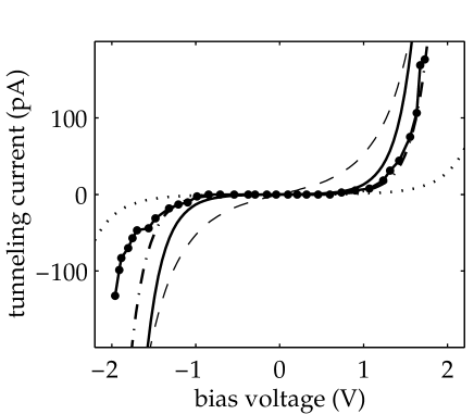
FIG. 1.: The $J-V$ characteristics of a 1.46 nm wide and 1.85 eV high MIM junction (the height measured from the equilibrium chemical potential) [19]. The experimental results by Haraichi et al. [5] (solid-dotted) is compared with the computations within the NOR (solid), NOR with a 6 $\%$ increase of the width (dash-dotted), OR (dashed) and Simmons formula (dotted) [7]. The equilibrium chemical potential is 1.75 eV and the conduction band width is $2W=40$ eV.

REFERENCES

- [1] R.J.M. Vullers et al., Appl. Phys. Lett. 76, 1947 (2000).
- [2] M. Nakayama et al., Jap. J. Appl. Phys. 38, 7151 (1999).
- [3] B. Irmer et al., Appl. Phys. Lett. 71, 1733 (1997).
- [4] K. Mastumoto et al., Appl. Phys. Lett. 68, 34 (1996).
- [5] S. Haraichi et al., J. Vac. Sci. Technol. B 15, 1406 (1997).
- [6] L.I. Glazman and A.V. Khaetskii, Europhys. Lett. 9, 263 (1989).
- [7] J.G. Simmons, J. Appl. Phys. 34, 1793 (1963), ibid. 34, 1828 (1963).
- [8] J. Bardeen, Phys. Rev. Lett. 6, 57 (1961).
- [9] M.C. Payne, J. Phys. C 19, 1145 (1986).
- [10] A.I. Larkin and K.A. Matveev, Sov. Phys. JETP 66, 580 (1987).
- [11] Y. Meir and N.S. Wingreen, Phys. Rev. Lett. 68, 2512 (1992).
- [12] A-P Jauho et al., Phys. Rev. B 50, 5528 (1994).
- [13] A.V. Svidisinskii, Space-non-homogeneous Problems in Superconductivity (Nauka, Moscow, 1982) in russian.
- [14] E. Emberly and G. Kirczenow, Phys. Rev. Lett. 81, 5205 (1998).
- [15] J. Fransson, O. Eriksson, B. Johansson and I. Sandalov, Physica B 272, 28 (1999).
- [16] I. Sandalov and V.I. Filatjev, Physica B 162, 139 (1990).
- [17] L.P. Kadanoff and G. Baym, Quantum Statistical Mechanics (Benjamin, New York, 1962).
- [18] D.C. Langreth, in Linear and nonlinear electron transport in solids, Vol. 17 of Nato Advanced Study Institute, Series B: Physics, edited by J.T. Devreese and V.E. van Doren (Plenum, New York, 1976).
- [19] The experimental data of the barrier’s width and height given by Haraichi et al. [5] are calculated from , which is only valid for low and intermediate voltages. In the Fig 1, we have used the more precise . The two formulae for the current are found in Ref. [7].
- [20] L.D. Landau and E.M. Lifshitz Quantum Mechanics 3 ed. (Pergamon Press 1977).