The dynamics of a strongly driven two component Bose-Einstein Condensate.
Abstract
We consider a two component Bose-Einstein condensate in two spatially localized modes of a double well potential, with periodic modulation of the tunnel coupling between the two modes. We treat the driven quantum field using a two mode expansion and define the quantum dynamics in terms of the Floquet Operator for the time periodic Hamiltonian of the system. It has been shown that the corresponding semiclassical mean-field dynamics can exhibit regions of regular and chaotic motion. We show here that the quantum dynamics can exhibit dynamical tunneling between regions of regular motion, centered on fixed points (resonances) of the semiclassical dynamics.
I Introduction
Since the first experimental realization of a Bose condensed gas of atoms in 1995 [1] there has been considerable interest in the properties of Bose-Einstein Condensates (BEC’s). Here we are interested in the properties of a BEC confined to the two spatially localized regions of a double well potential, and subjected to periodic modulation in such a way that the tunnel coupling between the two wells is periodically modulated. In this way it has been shown that the semiclassical mean-field dynamics can exhibit regions of chaotic motion [2, 3].
The primary goal of this paper is to develop an understanding of the quantum dynamics, beyond mean-field theory, of a dynamical system in a classically chaotic regime. In particular we seek quantum features of the dynamics of strongly driven BEC’s that are not obtained in mean-field theory. Over the last two decades there have been numerous studies of nonlinear systems with a finite number of degrees of freedom; a topic that is often referred to as ‘quantum chaos’, see for example [4, 5]. In this paper however we attempt to address the quantum dynamics of a driven quantum field. In the mean-field limit, an effective classical field (a system of an infinite number of degrees of freedom) is used to describe the condensate. The response of the system to external periodic forcing would then be described by the driven Gross-Pitaevskii equation. In the hydrodynamic limit the mean field description would look very much like a forced nonlinear fluid dynamics model [6]. A similar system of equations also arise in periodically modulated nonlinear optical fibers [7]. Even without external time dependent forcing nonlinear field equations of the kind considered here exhibit dynamical instabilities leading to a host of interesting phenomenon for both the integrable case (e.g. solitons) and the non-integrable case (e.g. turbulence) [8, 9]. The response of condensates to forcing can encompass a large variety of physical situations including vortex formation in response to stirring [10], and rotating condensates in an anisotropic trap [11]. Adhikari [12] recently conducted a numerical study, in mean field theory, of two couple condensates with modulation of the trap frequency and also modulation of the nonlinear term due to hard sphere collisions. Gardiner et.al. [13] considered a BEC in a modulated periodic potential.
We will consider two condensates with a tunnel coupling periodically modulated in time. In a fully quantum treatment the dynamics is given by a nonlinear equation for the field operator. We do not know in general how to deal with such systems. In this paper we adopt the usual method of a finite mode expansion, which effectively reduces both the classical and quantum systems to systems with few degrees of freedom. Even at this crude level of approximation however we can find fundamental differences between the mean-field predictions and those of the quantum description.
In this paper we focus on two tunnel-coupled BEC’s in a double well potential, including the nonlinear self energy term, with periodic modulation of the tunnel coupling. A similar model has recently been studied by Abdullaev and Kraenkel [3] in the mean-field limit. They also included modulation of the energy difference between the two condensates as well as dissipation. They showed that, in mean-field theory, the system could exhibit chaotic oscillations of the relative population difference between the two wells. Recently, Elyutin and Rogovenko have treated a periodically driven double well model via the Gross-Pitaevskii equation [21]. There are many studies of a BEC in a time independent double well potential [14, 15, 16, 17, 18, 19, 20]. We will use the model of reference [18] which is valid for small condensates (few atoms, i.e. ), where one expects quantum departures from mean-field theory to be more significant. We make a two mode approximation for the double well system [18, 22, 23], with weak interwell tunneling. As particle number is a constant of the motion at zero temperature, we can use an approach based on the two mode bosonic realization of the SU(2) algebra. We use the Schrödinger picture and an angular momentum model for the quantum system in SU(2) dynamics. We find a parameter regime in which an initial atomic coherent state tunnels from one fixed point (resonance) to another. This behavior is analyzed from a Floquet state perspective and reveals an interesting feature of parity of the Floquet operator eigenstates.
The many body Hamiltonian is specified in section II, and our two mode approximation to it is given. Section III outlines the models and the corresponding equations of motion for the two mode system. The semiclassical and quantum results are discussed in sections IV and V respectively, followed by our concluding remarks in section VI.
II The Hamiltonian
The many-body Hamiltonian for an atomic BEC confined in a potential is given by [24],
| (1) |
where is the boson mass, measures the strength of the two body interaction and is the s-wave scattering length. and are the Heisenberg creation and annihilation operators of particles at position . , and . is a time dependent potential, parameterised by the modulation strength , and the driving frequency . Throughout this paper implies non-driven dynamics and corresponds to driven (modulated) dynamics.
We will follow the model of reference [18] in which the trap potential is taken to be a symmetric double well in the -direction and harmonic in the -directions,
| (2) |
where is the trap frequency in the plane, and where gives the strength of the confinement in the -direction. The potential has stable fixed points at near which the linearised motion is harmonic with frequency . For simplicity we will set . The length scale is set by the rms position fluctuations, , in the ground state of the harmonic potential near the fixed points; . In terms of this parameter the barrier height separating the two wells may be written .
We assume the potential is such that there are two nearly degenerate single particle energy eigenstates below the barrier and expand the field in terms of two localised single particle states, , at each stable minima;
| (3) |
where is defined to be the normalized single-particle ground state mode of the harmonic potential near each stable fixed point, , each with energy . The details can be found in [18]. The energy eigenstates of the double well may then be approximated as symmetric () and antisymmetric () combinations of the localised states with energy eigenvalues given in first order perturbation theory by where the energy level splitting determines the tunnelling frequency and is given by
| (4) |
As discussed in [18] the validity of the two mode approximation requires .
The effect of the modulation is to directly modulate the parameter so that it becomes . This has two important effects; it modulates the harmonic frequency around each fixed point and it modulates the tunnelling frequency, so that these quantities become time dependent , where
| (5) | |||||
| (6) |
The two mode approximation then results in the following Hamiltonian [18],
| (7) | |||||
| (8) |
where
| (9) |
and similarly for , . and are creation and annihilation operators for atoms in the local modes in wells 1 and 2 respectively. The remaining parameters in the Hamiltonian are as follows, represents the particle-particle interaction and measures the tunnelling rate of atoms between wells 1 and 2. We will assume that the system remains in a total number eigenstate, with eigenvalue . We first note that we will be interested in modulation frequencies that are of the order of the unmodulated tunnelling frequency, . The condition for the validity of the two mode approximation then ensures that . We can then replace the first term in the Hamiltonian by a slowly varying number , which has no influence on the quantum dynamics. The temporal modulation of the second term, which is responsible for tunnelling, has a strong influence on the dynamics as we show.
If is small enough we can approximate the modulated tunnelling frequency by
| (10) |
where . While may be small we cannot necessarily claim that is small. We may expand the approximate expression for using Fourier series,
| (11) |
where is a Bessel function. In general we see that the direct modulation of the potential leads to a non-harmonic modulation of the tunnelling frequency. In what follows we will neglect the higher harmonics of the modulation frequency, and consider the time dependence of to be simply
| (12) |
While we have assumed that is small, this constraint is not as strong as one might expect. When we study the ratio of the approximate modulated tunnelling to the complete expression given in Eq.(6), , we find that for appropriate values of , the ratio is close to unity even for values of as large as . Henceforward we will assume the simpler harmonic modulation of .
The separation of the higher excited states from the nearly degenerate ground states is of the order of . As the validity of the two mode approximation requires that , and we assume that the driving frequency is of the order of the tunnelling frequency. The driving frequency is very far from resonance with higher excited states of the double well and we can continue to make a two level approximation when the modulation is present. Of course when the tunnelling and the modulation is slow, the interesting dynamics will occur on a long time scale and one may legitimately ask if dissipation should not be included. In this paper however we will neglect the effect of dissipation and focus only on the nonlinear quantum dynamics. Our results are thus strictly only valid for zero temperature. The validity of an expansion in terms of localised single particle states places a restriction on the atomic number [18]. We are thus only concerned with very small condensates at temperatures low enough that the non-condensate fraction, and the resulting dissipation, can be neglected. It is only in this regime that quantum (rather than semiclassical) nonlinear effects in driven BEC’s could be observed.
Using the generators for SU(2) dynamics,
| (13) | |||||
| (14) | |||||
| (15) |
the two mode Hamiltonian may be written,
| (16) |
It is worth noting the symmetry of this Hamiltonian under parity reflection of . The dynamics of this two mode system are greatly simplified by this symmetry.
The operator represents the difference in atom number between wells 2 and 1 while the total number of atoms is given by . As a consequence of number conservation, the operators of Eqs.(13,14,15) have a Casimir invariant given by
| (17) |
and are of no particular significance for our present purposes and are not considered further.
III The Equations of Motion
In reference [18] the mean-field equivalent of the two mode approximation used here was shown to result from a moment factorization ansatz in the Heisenberg equations of motion. In effect this is equivalent to a classical two mode approximation for the Gross-Pitaevskii equation. We start by using the Heisenberg equation of motion to find the time evolution of the three operators in Eqs.(13,14,15). Using the familiar commutation relations , we obtain three equations of motion for the operators and .
| (18) |
| (19) |
| (20) |
We transform these Heisenberg equations of motion into a semiclassical system of equations by taking the expectation value of the above equations and factorizing operator products such as . This leaves us with classical numbers in place of the operators. We make the identification , i.e. we scale the equations by the total number of atoms N. We now write down the semiclassical system of scaled equations,
| (21) | |||||
| (22) | |||||
| (23) |
with the usual constraint to the sphere,
| (24) |
We identify three real variables , corresponding to the operators ,
| (25) |
| (26) |
| (27) |
where the ’s are c-numbers, and are the expectation values of the second quantized annihilation and creation operators . These real variables can be shown to represent the following physical parameters, represents the difference in atom number between wells 2 and 1, represents the momentum of the condensate and represents the population difference between the global symmetric and antisymmetric modes of the confining potential [18].
IV Semiclassical Dynamics
While we can imagine a vector tracing out some trajectory on the surface of the sphere, see Fig. 1., it is convenient to make a stereographic projection of the dynamics onto a two dimensional plane.
We use a stereographic projection of a sphere onto the plane via the transformation,
| (28) |
Using the definitions and we write,
| (29) |
| (30) |
Setting , we rewrite the system of Eqs.(21,22,23) as,
| (31) | |||||
| (32) |
Where we have scaled the time by and we set . The equator of the sphere is mapped to the unit circle in (a,b) phase space due to our choice of radius () for the sphere and the position of the wells are mapped to .
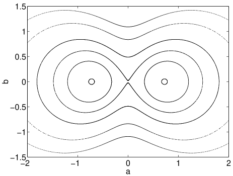
For , i.e. , the system (32) is integrable. If , the only feature is a center at the origin. At , the origin undergoes a pitchfork bifurcation creating two stable centers, which for have position
| (33) |
and are surrounded by a ‘figure 8’ type separatrix. The integral curves for this system are,
| (34) |
On the separatrix , for solutions to Eq.(34) lie inside the separatrix and for they lie outside.
Fig. 2. shows the phase plane for , illustrating the integral curves. If we consider starting in one well, say , then for , complete population oscillations between the wells occur [18]. At we find the separatrix intersects the centers of the wells and complete oscillations no longer occur. As increases beyond (larger , i.e. more atoms) the solutions of Eqs.(32) become localized near the fixed points of the phase plane. This is known as self-trapping. Physically, this can be interpreted as an increase in the self energy with particle number which modifies the effective single particle potential of the system and reduces the single particle tunneling [18].
A very similar model with harmonic driving is considered by Elyutin and Rogovenko [21]. In that paper they find fixed points and a separatrix for their model analagous to the fixed points and separatrix in the model treated here. They consider the break down of the regular phase space due to the overlap of resonances, and show tunnelling between the classical fixed points of the semiclassical phase space. We go a step further here in that direction firstly to analyze the dynamics of fixed points of the Poincaré map (resonances) and initial conditions localized on those semiclassical resonances and secondly to analyze a full quantum description.
Resonances
For the modulated tunneling rate gives rise to resonances. Outside the separatrix, a resonance will appear when there is a rational ratio between the driving period and the period of motion of the system on a given integral curve. We know on a particular integral curve , the system period is given by,
| (35) |
where is a complete elliptic integral of the first kind, and are given by
| (36) |
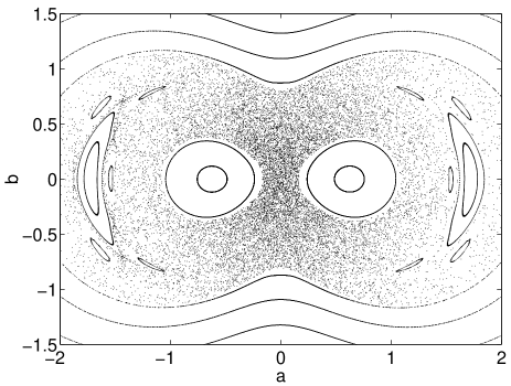
In particular, the integral curve given by is resonant, breaking up under perturbation to give two stable period-1 resonances which for lie on the momentum axis. These can be seen in the Poincaré section, , which here is simply a stroboscopic map taken at . In such a stroboscopic map, see Fig. 3., the resonances appear as fixed points. They lie outside the separatrix, which has been replaced by a ‘chaotic sea’, and are distinct from the two period-1 fixed points nearer the origin. For , here it was taken as 1.37, these period-1 resonances exist for .
In order to make a comparison with the quantum dynamics we need to consider an initial classical distribution rather than a single point, and compute average values of the dynamical variables as the distribution evolves in time. The classical phase space density (distribution) we require to simulate the quantum state must correspond to a system of points localized on the spherical classical phase space and should describe the optimal simultaneous determination of the phase space variables, that is the components of angular momentum. These states are known as the SU(2) coherent states [25] and are defined in Eq.(42).
For a quantum state , the distribution that describes the output for optimal simultaneous measurement of angular momentum is
| (37) |
where . If the system begins in an initial SU(2) coherent state , the corresponding distribution is [26]
| (38) |
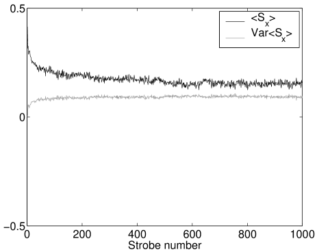
where is the total angular momentum quantum number. This is the classical distribution that we sample to compute the ensemble dynamics. The distribution is normalized with respect to the spherical integration measure, which in the stereographic coordinates is . If we start an initial distribution of points in a stable resonance island, the population remains confined by the invariant tori bounding the island, see Fig. 4. In the next section we shall see how the equivalent quantum simulations produce a very different result.
V Quantum Dynamics
It is difficult to solve nonlinear Heisenberg equations of motion so we work in the Schrödinger picture using an orthonormal basis defined by the eigenstates of , as in [18]. Using the familiar angular momentum notation we write our state as,
| (39) |
and substitute into the Schrödinger equation to get
| (40) |
This is a set of linear coupled equations ( of them) and we use a Runge-Kutta numerical routine to solve them for the coefficients . Given these coefficients we can obtain the various expectation values and thus the solution of our model. We once again treat the driven and undriven systems separately. For we obtain regular collapse and revival sequences as shown previously in [18].
For the system is described by a time periodic Hamiltonian. In that case the appropriate description is in terms of the Floquet operator , of the system which maps the state from one time to a time exactly one modulation period later [5],
| (41) |
The Floquet map is the quantum equivalent of the classical Poincaré section defined in section IV. We obtain the Floquet Operator in the basis which diagonalizes as follows. Solve the Schrödinger equation over one modulation period of time to obtain for the set of initial conditions . The solution vectors, , form the columns of the Floquet Operator matrix .
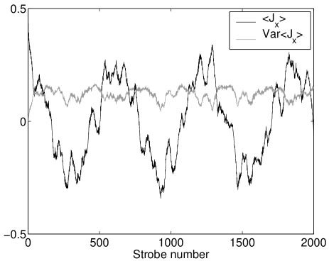
In Fig. 5., we plot the mean value of for an initial state localized on the same period-one resonance as in Fig. 4. We use the SU(2) coherent states as the initial localized states. These are defined on the sphere by [18],
| (42) |
where , and and are the spherical polar coordinates. For the parameters it is found that after modulation periods, the system state appears to be localized on the other resonance, see Fig. 5. This behavior is known as dynamical tunneling [27]. Dynamical tunneling is a different process from the well-known case of barrier tunneling. There is no energetic or potential barrier. None the less in dynamical tunneling the system exhibits classically forbidden motion, motion which cannot be accessed by a classical particle moving on any trajectory. Dynamical tunneling in a single atom system has recently been observed by two groups [28, 29].
We can understand the tunneling in the following way. The Hamiltonian is invariant under rotations about the z-axis, i.e. operations of leave the Hamiltonian unchanged. Thus the Floquet states, by the nature of their construction must fall into two sets, corresponding to the eigenvalues of . These two sets contain vectors of odd and even parity.
Let be a state localized on one of the period-one resonances with coordinates , while , is localized on the other period one resonance, . These states are related by a rotation of by about the axis,
| (43) |
As the Hamiltonian is invariant under rotations of around the z axis, the eigenstates of the Floquet operator fall into two parity classes defined by this rotation. If the initial state is well localized on one of the period-one resonances, it will tend to have maximal support in a two dimensional subspace spanned by two particular Floquet eigenstates of opposite parity. We label these two simultaneous eigenstates of and parity as , where are the corresponding eigenvalues of the Floquet operator. We then write the ‘negative’ and ‘positive’ localized states, as a superposition of these parity eigenstates states, i.e.
| (44) |
and,
| (45) |
where are very nearly equal and together almost exhaust the normalization condition, .
For complete tunneling we must have, . How many iterations of Eq.(41) satisfy this tunneling condition? Suppose we start in the state . After iterations of the Floquet map we reach the state
| (46) |
When the relative phase of the two states in this superposition is shifted by , the state becomes almost equal to a state localized in the other period-one resonance . This determines the tunneling time as
| (47) |
To find the particular Floquet eigenstates on which an initially localized state has maximum support we simply expand the initial state in the basis of Floquet eigenstates. This also gives the corresponding eigenphases and thus the tunneling time. By this method we find the tunneling time should be . This compares favorably with the tunneling time of about evident in Fig. 5.
We expect to see the variance of at a minimum whenever the component is most localized around each of the resonances, which is when the state should be close to a minimum uncertainty state. At the half way point, a coherent superposition of two states of equal and opposite mean values of should occur, and the variance should be a maximum. This behavior is evident in Fig. 5.
VI Conclusion
In this paper we have used a two mode approximation to describe the quantum dynamics of a BEC in a double well potential with periodic modulation of the potential barrier separating the two wells. In mean-field theory (Gross-Pitaevskii limit) we find, for appropriate parameter values, a mixed phase space of regular stable motion, associated with fixed points, coexisting with chaotic dynamics. We have shown the existence of dynamical quantum tunneling between period-one fixed points (resonances). This dynamical tunneling is distinct from the single particle tunneling present in the undriven system and may be interpreted as a new signature of the quantum dynamics of a nonlinear quantum field.
Double well potentials similar to those modeled here have been experimentally realized, see for example [16, 28, 30]. While current experiments are unlikely to be well described by the two mode model given here, we expect dynamical tunneling to be sufficiently robust that an experimental realization of the dynamical quantum tunneling predicted here can be observed. The recent observation by the NIST group [29] of dynamical tunneling of a single particle system in a modulated periodic potential in fact used a BEC, although not in a regime where the mean-field is significant. It would not be difficult to modify the experiment so that the nonlinear effect of the BEC would be significant.
Acknowledgements
G.L.S. wishes to thank Kae Nemoto and Bill Munro for very helpful discussions.
REFERENCES
- [1] M. H. Anderson, J. R. Ensher, M. R. Matthews, C. E. Wieman and E. A. Cornell, Science 269, 198 (1995).
- [2] G. J. Milburn, J. Corney, D. Harris, E. M. Wright and D. F. Walls, Atom Optics: Proceedings of SPIE 2995, 232 (1997).
- [3] F. K. Abdullaev and R. A. Kraenkel, Phys. Rev. A 62 023613 (2000).
- [4] H. -J. Stöckmann, Quantum Chaos - An Introduction, Cambridge University Press (1999).
- [5] F. Haake, Quantum Signatures of Chaos, Springer-Verlag (1991).
- [6] S.Stringari, Phys. Rev. A 58, 2385 (1998).
- [7] C. Sulem and P. -L. Sulem, , The nonlinear Schrödinger equation; self focusing and wave collapse, Applied Mathematical Sciences, 139, Springer, New York, (1999).
- [8] D. Cai and D. W. Laughlin, J.Math. Physics, 41, 4125 (2000).
- [9] D. Cai, D. W. McLaughlin, K. T. R. McLaughlin, The Nonlinear Schrödinger Equation as Both a PDE and a Dynamical System, citeseer.nj.nec.com/cai00nonlinear.html (2001).
- [10] J. Brand and W. P. Reinhardt, J. Phys. B 34, L113 (2001).
- [11] S. Sinha and Y. Castin Phys. Rev. Lett. 87, 190402 (2001).
- [12] S. K. Adhikari, Phys. Rev. E 63, 056704 (2001).
- [13] S. A. Gardiner, D. Jaksch, R. Dum, J. I. Cirac and P. Zoller, Phys. Rev. A 62, 023612 (2000).
- [14] J. Javanainen, Phys. Rev. Lett. 57, 3164 (1986).
- [15] F. Dalfovo, L. Pitaevskii and S. Stringari, Phys. Rev. A 54, 4213 (1996).
- [16] M. R. Andrews, C. G. Townsend, H. -J. Miesner, D. S. Durfee, D. M. Kurn and W. Ketterle, Science 275, 637 (1997).
- [17] A. Smerzi, S. Fantoni, S. Giovanazzi and S. R. Shenoy, Phys. Rev. Lett. 79, 4950 (1997).
- [18] G. J. Milburn, J. Corney, E. M. Wright and D. F. Walls, Phys. Rev. A 55, 4318 (1997).
- [19] S. Raghavan, A. Smerzi, S. Fantoni and S. R. Shenoy, Phys. Rev. A, 59, 620 (1999).
- [20] E. A. Ostrovskaya, Y. S. Kivshar, M. Lisak, B. Hall, F. Cattani and D. Anderson, Phys. Rev. A 61, 031601 (2000).
- [21] P. V. Elyutin and A. N. Rogovenko, Phys. Rev. E 63, 026610 (2001).
- [22] R. W. Spekkens and J. E. Sipe, Phys. Rev. A. 59, 3868 (1999).
- [23] J. I. Cirac, M. Lewenstein, K. Mølmer and P. Zoller, Phys. Rev. A 57, 1208 (1998).
- [24] A. Griffin, D. W. Snoke and S. Stringari (eds.), Bose-Einstein Condensation, Cambridge University Press (1995).
- [25] D. M. Appleby, Int. J. Theor. Phys. 39, 2231 (2000).
- [26] B. C. Sanders, Phys. Rev. A 40, 2417 (1989).
- [27] M. J. Davis and E. J. Heller, J. Chem. Phys. 75, 246, (1981).
- [28] D. Steck, W. H. Oskay and M. G. Raizen, Science 293, 274 (2001)
- [29] W. K. Hensinger, H. Häffner, A. Browaeys, N. R. Heckenberg, K. Helmerson, C. McKenzie, G. J. Milburn, W. D. Phillips, S. L. Rolston, H. Rubinsztein-Dunlop and B. Upcroft, Nature 412, 52 (2001).
- [30] K. B. Davis, M. -O. Mewes, M. R. Andrews, N. J. van Druten, D. S. Durfee, D. M. Kurn, and W. Ketterle, Phys. Rev. Lett. 75, 3969 (1995).