ARPES in the normal state of the cuprates: comparing the marginal Fermi liquid and spin fluctuation scenarios

Abstract

We address the issue whether ARPES measurements of the spectral function $A_{k}(\omega)$ near the Fermi surface in the normal state of near optimally doped cuprates can distinguish between the marginal Fermi liquid scenario and the spin-fluctuation scenario. We argue that the data for momenta near the Fermi surface are equally well described by both theories, but this agreement is nearly meaningless as in both cases one has to add to $\Sigma^{\prime\prime}(\omega)$ a large constant of yet unknown origin. We show that the data can be well fitted by keeping only this constant term in the self-energy. To distinguish between the two scenarios, one has to analyze the data away from the Fermi surface, when the intrinsic piece in $\Sigma(\omega)$ becomes dominant.

The observed discrepancies between the normal state properties of the cuprates and the predictions of Fermi liquid theory continue to attract a lot of attention from the condensed-matter community. In a Fermi liquid, the quasiparticle damping near the Fermi surface behaves as $\omega^{2}$ or $(\pi T)^{2}$, whichever is larger. This gives rise to the $\omega^{2}$ ($T^{2}$) behavior of the width of the peak in the quasiparticle spectral function $A_{k}(\Omega)=(1/\pi)ImG(k,\Omega)$ measured in the angle-resolved photoemission (ARPES) experiments.

The data on optimally doped cuprates show several features which are in disagreement with Fermi liquid theory: $\Sigma^{\prime\prime}(\omega,T)$ is large and does not display a Fermi liquid form for all $T>T_{c}$ and for all frequencies. Instead, over a wide range of $\omega$ and $T$, $\Sigma^{\prime\prime}(\omega,T)$ resembles a linear function of both arguments [1, 2, 3, 4]. As a result $\Sigma^{\prime\prime}(\omega,T)$ does not become progressively smaller than $\omega$ with decreasing $\omega$, and the spectral function does not undergo a drastic sharpening at the smallest energies, as it does in a Fermi liquid. Whether this effect is quantitative or qualitative is still a matter of debate as in the normal state experiments, $T$ remains finite and larger than $T_{c}$. The data for overdoped materials do show a stronger sharpening of the spectral function near $k_{F}$ indicating that these materials are likely Fermi liquids [5]. From this perspective, the unusual behavior of optimally doped cuprates indicates that the upper energy cutoff for the Fermi liquid behavior rapidly reduces down from the Fermi energy. This is a typical situation for system near a quantum phase transition.

In this communication, we compare two scenarios for the non-Fermi liquid behavior, both are based on the idea of quantum criticality. The first is the marginal Fermi liquid (MFL) scenario developed in Ref [6]. This scenario assumes that there exists a quantum-critical point (QCP) separating the Fermi liquid and the pseudogap regimes (Fig. 1a). Superconductivity develops in the shaded region about the QCP. In the quantum-critical regime, the system is assumed to display a marginal Fermi liquid behavior with

$$\Sigma^{mfl}_{\mathbf{k}}(\omega)=-\lambda_{mfl}[\omega\log(\frac{\omega}{\omega_{0}})-i\frac{\pi}{2}\sqrt{\omega^{2}+\pi^{2}T^{2}}]$$ (1)

where $\lambda_{mfl}$ and $\omega_{0}$ are the two adjustable parameters. To satisfy Kramers-Kronig relations, $\omega_{0}$ should possess a nonsingular dependence on $(\pi T/\omega)^{2}$, but this dependence is usually neglected. The self energy is defined such that $G({\mathbf{k}},\omega)=1/(\omega-\epsilon_{\bf k}+\Sigma({\bf k},\omega))$. We plot $\Sigma^{mfl}(\omega)$ in Fig. 1b and c. This marginal behavior naturally emerges near the critical points in $3D$, however obtaining this behavior in 2D systems is still problematic. To do so, it is possible that special requirements such as, e.g., singular momentum dependence of the low-energy bosonic mode which mediates the fermionic interaction [7] must be satisfied.

Another scenario is based on the idea that the dominant interaction in the cuprates is between fermions and their low-energy collective spin excitations. This physics is described by the spin-fermion (SF) model.  [8, 9] In this scenario, the non-Fermi liquid behavior in the normal state is also associated with the closeness to a critical point, but this point now separates paramagnetic and antiferromagnetically ordered phases. The pseudogap phase emerges in the SF model as a dome around this critical point, and optimal doping roughly corresponds to a situation when this dome intersects the crossover line separating Fermi liquid and quantum-critical regions (see Fig. 1d). Superconductivity results in the shaded region where the pseudogap and Fermi liquid regimes intersect, and the normal state non-Fermi liquid behavior occurs in the quantum critical regime that near optimal doping stretches down to almost $T_{c}$. The quantum-critical behavior in the SF model has been analyzed in detail. [9] The model has two parameters; $\omega_{sf}$ which is the typical frequency for the relaxational spin dynamics and also turns out to be the upper cutoff of the Fermi liquid behavior, and the dimensionless coupling $\lambda_{sf}$. Both $\lambda_{sf}$ and $\omega_{sf}^{-1}$ increase as the system approaches a magnetic instability, but the product ${\bar{\omega}}=4\lambda_{sf}^{2}\omega_{sf}$ remains finite and serves as the upper cutoff for the quantum-critical behavior. The separation into Fermi liquid and quantum critical regions makes sense when $\lambda_{sf}\geq 1$ or equivalently when $\omega_{sf}\ll{\bar{\omega}}$. In general, $\lambda_{sf}$ and $\omega_{sf}$ (but not ${\bar{\omega}}$) depend on the momenta along the Fermi surface, but this dependence is rather mild as we will show.

The microscopic nature of the SF model implies that the self-energy is totally determined and has to be obtained in explicit calculations. At $T=0$, the Eliashberg-type calculations yield

$$\Sigma^{sf}_{\mathbf{k}}\left(\omega\right)=\lambda_{sf}~{}\frac{2\omega}{1+\sqrt{1-i\frac{\left|\omega\right|}{\omega_{\mathrm{sf}}}}}$$ (2)

At small frequencies, $\omega\ll\omega_{\mathrm{sf}}$, $\Sigma^{sf}_{\mathbf{k}}\left(\omega\right)=\lambda_{sf}\left(\omega+i\omega\left|\omega\right|/4\omega_{\mathrm{sf}}\right)$ and the system displays a Fermi liquid behavior. At frequencies above $8-10\omega_{\mathrm{sf}}$, the fermionic self-energy displays a quantum-critical behavior, in which ${\bar{\omega}}$ is the only energy scale: $\Sigma^{sf}_{\mathbf{k}}\left(\omega\right)=e^{i\pi/4}\mathrm{sign}\omega~{}\left(\bar{\omega}|\omega|\right)^{1/2}$. At intermediate frequencies, $\Sigma^{sf}_{\mathbf{k}}\left(\omega\right)$ interpolates between the two limits. Although there is no intermediate asymptotic (i..e., the crossover happens at energies $O(\omega_{sf})$), the intermediate regime is rather wide, and in between $\omega_{sf}/2$ and at least $6-8\omega_{sf}$, $\Sigma_{\mathbf{k}}^{sf}\left(\omega\right)$ resembles a linear function of $\omega$. The finite temperature result is more complicated [9] but posesses the same basic characteristics as the zero temperature result. We plot $\Sigma_{\mathbf{k}}^{sf}\left(\omega\right)$ at $T=100K$ in Fig. 1d.

In light of the strong simliarities between the MFL and SF fermionic self energies, it is important to ask which experiments allow us to distinguish between the two scenarios. We focus in this communication on energy distribution curve (EDC) ARPES experiments performed for momenta near the Fermi surface. Abrahams and Varma [10] have argued that such ARPES experiments help put strong constraints on the form of the pairing interaction and can rule out many of the scenarios for the non-Fermi liquid behavior in the normal state. In particular, they argued (i) that the MFL form of $\Sigma(\omega)$ nicely fits the experimental data, and (ii) the data along the Fermi surface can be fitted assuming that the MFL coupling $\lambda_{mfl}$ is almost independent of the position on the Fermi surface. They argued that this rules out a magnetic scenario since the bosonic interaction is peaked at $Q=(\pi,\pi)$ and hence the coupling constant should be momentum dependent with the maximum at hot spots (points at the Fermi surface separated by $Q$) in contradiction with (ii). We, on the contrary, demonstrated previously [11] that the photoemission data near $(0,\pi)$ and along the zone diagonal can be well fitted by the spin-fluctuation self-energy, Eq. (2), with $\lambda_{sf}$ varying along the Fermi surface.

We re-examine this issue using recent photoemission results from the Argonne group. [16] We will argue that EDC data for $k\approx k_{F}$ can be reasonably well fitted by both the MFL and SF theories, but the way in which the fitting works poses a serious question for both scenarios. Namely, in both fits, one has to add to the self-energy a large imaginary constant $i\gamma({\vec{k}}_{F})$ of yet unknown origin. We show that the fits with $\Sigma_{k}(\omega)=i\gamma({\vec{k}}_{F})$ with no frequency dependent terms added turn out to be of the same quality as the fits with $\Sigma^{full}_{k}(\omega)=\Sigma_{k}(\omega)+i\gamma$ where $\Sigma_{k}(\omega)$ has either MFL or SF form. From this perspective, the ARPES measurements near the Fermi surface do not allow the ruling out of either scenario. The situation may be different at large deviations from $k_{F}$ when the maximum in the photoemission intensity moves to high frequencies, and $\Sigma_{k}(\omega)$ (which increases with $\omega$) becomes larger than $\gamma$. In this case, one could possibly distinguish between MFL and SF scenarios by examining both the frequency dependence of $\Sigma^{\prime\prime}(\omega)$ and the sign and magnitude of $\Sigma^{\prime}(\omega)$.

Before we proceed with the fitting, we briefly review the experimental setup [1, 2, 4, 12, 14, 13, 15]. Two types of ARPES experiments are currently available. The EDC (energy distribution curve) experiments measure fermionic $I_{k}(\omega)=A_{k}(\omega)n_{F}(\omega)$ as a function of frequency at a given $k$. The MDC (momentum distribution curve) experiments measure $I_{k}(\omega)$ as a function of $k$ transverse to the Fermi surface at a given frequency. In general, near the Fermi surface,

$$A_{k}(\omega)=\frac{1}{\pi}\frac{\Sigma^{\prime\prime}_{k}(\omega)}{(\omega+\Sigma^{\prime}_{k}(\omega)-v_{k}(k-k_{F}))^{2}+(\Sigma^{\prime\prime}_{k}(\omega))^{2}}$$ (3)

There are both experimental and theoretical indications that in the cuprates, the fermionic self-energy is almost independent of the momentum component transverse to the Fermi surface although it strongly depends on frequency, and also possesses some dependence on the momentum along the Fermi surface. In this situation, the self-energy in the MDC measurements remains almost a constant, and the photoemission intensity evolves with $k$ as

$$I^{MDC}_{k}(\omega)\propto\frac{1}{(v_{F}(k-k^{*}(\omega)))^{2}+(\Sigma^{\prime\prime})^{2}}$$ (4)

where $k^{*}(\omega)=k_{F}-(\omega+\Sigma^{\prime}(\omega))/v_{F}$. We see that $I_{k}$ has a Lorentzian form with the maximum at $k=k^{*}$ and FWHM $|k-k^{*}|=\Sigma^{\prime\prime}(\omega)/v_{F}$. In other words, the MDC measurements allow one to directly infer the frequency dependence of the fermionic self-energy. If $v_{F}$ were known, the MDC measurements would also yield the magnitude of $\Sigma^{\prime\prime}(\omega)$. However to obtain $v_{F}$ is itself a problem as the MDC dispersion extracted from the peak position at low enough $\omega$ is $\omega(k)=v^{*}_{F}(k-k_{F})$ where $v^{*}_{F}=v_{F}(1+\partial\Sigma^{\prime}(\omega)/\partial\omega)$, hence measuring the dispersion at low frequencies one obtains a renormalized $v^{*}_{F}$, not a bare $v_{F}$ [2]. One could hope to extract $v_{F}$ from the dispersion at higher frequencies, where $\omega>\Sigma^{\prime}(\omega)$, and $v^{*}_{F}$ approaches $v_{F}$. However, it is not quite clear whether $\Sigma^{\prime}(\omega)$ can be fully neglected at energies where one can restrict with the linearized dispersion near the Fermi surface.

In the EDC experiments, one measures at small enough frequencies

$$I^{EDC}_{k}(\omega)\propto\frac{\Sigma^{\prime\prime}(\omega)}{(\omega-\omega(k))^{2}+(\Sigma^{\prime\prime}(\omega)/v^{*}_{F})^{2}}$$ (5)

In a Fermi liquid $\Sigma^{\prime\prime}(\omega)$ is small and near $\omega=\omega(k)$ can be approximated by a constant - its value at $\omega=\omega(k)$. $I^{EDC}_{k}(\omega)$ then has a Lorentzian form with FWHM $\Sigma^{\prime\prime}(\omega)/v^{*}_{F}$. As $v^{*}_{F}$ is directly measured from the dispersion, one could straightforwardly extract $\Sigma^{\prime\prime}(\omega)$ from the data. In the cuprates, however, the situation is more complex as (i) typical frequencies are not small, and hence $v_{F}^{*}$ itself depends on frequency, and (ii) $\Sigma^{\prime\prime}(\omega)$ is not small, and its frequency dependence matters. Both effects give rise to a non-Lorentzian form of $I^{EDC}_{k}(\omega)$, and the extraction of $\Sigma^{\prime\prime}(\omega)$ becomes problematic.

In Figs 2, 4 and 5 we present the data for $I_{k}(\omega)$ obtained from EDC experiments by Kaminski et al [16] taken at $100K$ from near optimally doped Bi2212 with a $T_{c}$ of $85K$. We have chosen lineshapes for two points near the Fermi surface, one is close to the zone diagonal ($k_{y}=0.54\pi/a$) , and another near a hot spot ($k_{y}=0.81\pi/a$). We see that the form of $I^{EDC}_{k}(\omega)$ is clearly different from a Lorentzian, even when the Fermi function is taken into account. In this situation, it is more reasonable to fit the whole $I^{EDC}_{k}(\omega)$ rather than the FWHM. This is what we will do.

In Fig.2 we present the theoretical fits using the MFL form of the self-energy. The fit in Fig. 2a is obtained using $\omega_{0}=500meV$. For this $\omega_{0}$, $\Sigma^{\prime}(\omega)$ is small at frequencies of few hundred meV (see Fig. 1) and to first approximation can be neglected. The fit in Fig. 2b is obtained using a deliberately large $\omega_{0}=5eV$, in which case the real part of the self-energy is strong. We see that both fits are rather good. The fitting parameters in Fig 2 a (b) are $\lambda_{mfl}=0.17(0.17)$, $\gamma=100(133)meV$ and $\epsilon_{k}=-26(-30)meV$ for $k$ along the zone diagonal, and $\lambda_{mfl}=0.15(0.15),\gamma=171(225)meV$, and $\epsilon_{k}=-43(-47)meV$ for $k$ close to a hot spot. To account for the flattening of the measured $I^{EDC}_{k}(\omega)$ at the highest frequencies, we also had to add a background contribution to $I^{EDC}_{k}(\omega)$ which we have chosen, following Ref. [10] to be just proportional to the Fermi function: $I^{EDC}_{k}(\omega)\rightarrow I^{EDC}_{k}(\omega)+\beta n_{F}(\omega)$. We found $\beta=1.57(1.64)$ along zone diagonal and $\beta=2.22(2.26)$ near the hot spots.

We next consider the fits by the SF model. As stated previously, the two input parameters in the model, $\omega_{sf}$ and $\lambda_{sf}$ generally depend on the momentum component along the Fermi surface. Near the hot spots, this dependence is universal and is given by $\lambda_{sf}(k)=\lambda_{sf}/Z^{1/2}_{k},~{}\omega_{sf}(k)=\omega_{sf}Z_{k}$ where $Z_{k}=1+(\delta k\xi)^{2}$, and $\xi$ and $\delta k$ are the spin correlation length and the momentum deviation from a hot spot along the Fermi surface, respectively [9]. The largest $\delta k\xi$ is for $\mathbf{k}$ along the zone diagonal. At optimal doping, ARPES measurements of the Fermi surface yield $\delta k^{\mathrm{\max}}\sim 0.2\pi/a\approx 0.6/a$ [1, 2]. The correlation length extracted from the NMR measurements [17] is $\xi\sim 1-2a$. Then $\lambda_{sf}$ is reduced by at most a factor of $2$ as one moves from hot spots to zone diagonal. For $\omega_{sf}$, the use of the expansion formula near hot spots would yield a bigger increase, but its actual variation is much smaller as the theoretical $\omega_{\mathrm{sf}}\propto\sin\phi_{0}$, where $\phi_{0}$ is the angle between Fermi velocities at $\mathbf{k}$ and $\mathbf{k}+\mathbf{Q}$, which tends to $\pi$ as $\mathbf{k}$ approaches the zone diagonal. [8] In Fig. 3 we present the results of a computation of $\omega_{sf}(k)$ along the Fermi surface which includes both of the above effects. The increase is only a factor of 2.4, consistent with the fact that $\omega_{sf}(k_{diag})$ extracted from fitting $v^{*}_{F}$ by the SF self-energy yields $\omega_{sf}(k_{diag})\sim 20-25meV$  [9] while the fits to NMR yield $\omega_{sf}\sim 15meV$ for fermions near hot spots [17]. For simplicity, in the SF fits, we will consider $\omega_{sf}$ to be independent of $k$ and set $\omega_{sf}=15meV$ in accordance with NMR. We, however, have verified that variations in $\omega_{sf}$ have little effect on ARPES lineshapes.

The fits using the SF form of the self-energy are presented in Fig 4. The two fits are obtained using momentum independent and momentum-dependent coupling $\lambda_{sf}(k)$, respectively. We see that the fits are of the same quality as those in Fig. 2. The fitting parameters in Fig 5 a (b) are $\lambda_{sf}=0.84(1.0)$, $\gamma=110(114)meV$, $\beta=1.68(1.63)$ and $\epsilon_{k}=-32(-30)meV$ for $k$ along the zone diagonal, and $\lambda_{sf}=0.84(1.5),\gamma=180(193)meV$, $\beta=2.31(2.28)$ and $\epsilon_{k}=-52(-45)meV$ for $k$ close to a hot spot. We verified that making $\lambda_{sf}$ a bit larger or allowing it to vary more over the Fermi surface does not change the accuracy of the fits.

Since the frequency dependence of the self energy appears to make little difference in the quality of the fits at the Fermi surface, we now attempt to fit the data by $\Sigma(\omega)=i\gamma(k)$ without extra MFL or SF frequency dependence. The results of these fits are presented in Fig.5. The fitting parameters are $\gamma=94meV$, $\beta=1.8$ and $\epsilon_{k}=-4.4meV$ for $k$ along the zone diagonal, and $\gamma=160meV$, $\beta=2.4$ and $\epsilon_{k}=-12meV$ for $k$ close to a hot spot. $\epsilon_{k}$ is much smaller than in the other two fits, due to the lack of a real part of the self energy in these fits.

All three fitting procedures work surprisingly well. The facts that the data are not obtained exactly at the Fermi surface (i.e., $\epsilon_{k}\neq 0$) and that one has to add the background do not differentiate between the fits and hence are not that relevant, particularly as $\epsilon_{k}\sim 50meV$ corresponds to a very small $|k-k_{F}|\sim\epsilon_{k}/v_{F}\sim 0.02(\pi/a)$. The two physically relevant parameters are the coupling constant $\lambda$ and the extra $\gamma(k)$. By adjusting $\gamma(k)$ one can fit the data quite well by both MFL and SF forms, and also by just $\Sigma^{\prime\prime}=i\gamma(k)$. This indicates that one cannot differentiate between theoretical scenarios by analyzing EDC data obtained near the Fermi surface. It is possible that the intrinsic piece of the self energy may be extracted by fitting either EDC or MDC at deviations from the Fermi surface of at least a few hundred meV. Finally, the large $\gamma(k)$ in the fits poses a problem for both MFL and SF scenarios. The origin of the $\gamma(k)$ is currently unknown and its understanding is clearly called for.

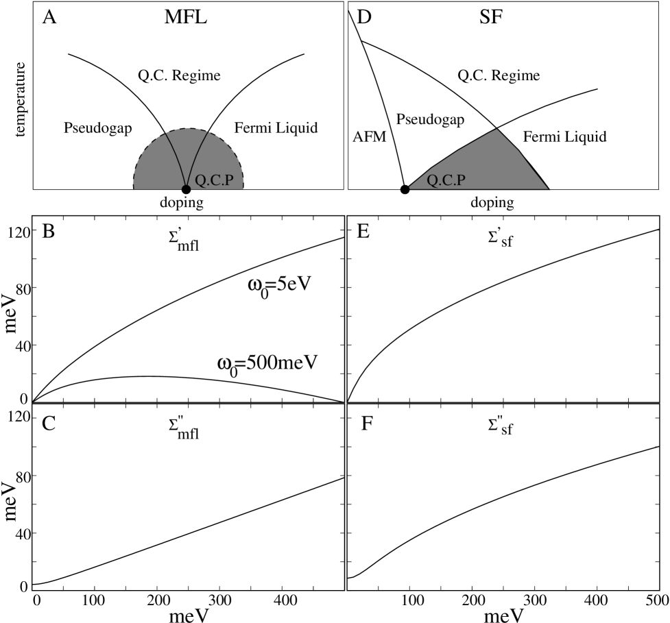
FIG. 1.: Comparison of the marginal fermi liquid and spin fermion scenarios. Figures a and d show the proposed phase diagrams for the MFL (a) and SF (d) pictures. Descriptions of the phase diagrams are in the text. Figures b,c and e,f compare the MFL and SF self energies at $T=100K$. Figures b and c show the real and imaginary parts of the MFL self energy respectively. $\lambda_{mfl}=0.1$ in both figures. In figure b, $\Sigma^{\prime}$ is given for both $\omega_{0}=500meV$ and $\omega_{0}=5eV$. Figures e and f show the real and imaginary self energies for the spin fermion model. $\lambda_{sf}=1.0$ and $\omega_{sf}=15meV$. $\Sigma^{\prime\prime}$ is seen to be roughly linear over a wide frequency range.

FIG. 2.: Fits of the measured EDC dispersion by the marginal Fermi liquid form of the self-energy. The intensity $I(\omega)$ is in arbitary units. The two fits have almost the same coupling $\lambda_{mfl}$ but different $\omega_{0}$ and different $\gamma$. In Fig. a, $\omega_{0}=500meV$ in which case the real part of the self-energy is small for the relevant frequencies. In Fig. b, $\omega_{0}=5eV$, and $\Sigma^{\prime}$ is relevant. Both fits work very well. The parameters are presented in the text.

FIG. 3.: The behavior of the spin-fluctuation frequency $\omega_{sf}$ along the Fermi surface. This frequency is the upper cutoff for the Fermi liquid behavior near an antiferromagnetic instability. We used $\epsilon(k_{x},k_{y})=-2t(\cos k_{x}+\cos k_{y})+4t^{\prime}\cos k_{x}\cos k_{y}-\mu$ with $t=250meV$, $t^{\prime}=-0.36t$, and $\mu=-1.1t$ chosen as being representative of optimal doping. The variation of $\omega_{sf}$ at a deviation from hot spots is determined by a competition between the increase due to a reduction of the magnetically mediated interaction, and the decrease due to the “nesting tendency” - the increase towards $\pi$ of the angle between the Fermi velocities at ${\bf k}_{F}$ and ${\bf k}_{F}+{\bf Q}$.

FIG. 4.: Fits of the measured EDC dispersion by the spin-fermion model with $\omega_{sf}=15meV$. (a) a fit using momentum independent coupling $\lambda_{sf}(k)=0.84$ for both the diagonal and the hot spot, (b) a fit using momentum dependent coupling $\lambda_{sf}=1.0$ along the diagonal and $\lambda_{sf}=1.5$ near the hot spots. Other parameters are presented in the text.

FIG. 5.: Fits of the measured EDC dispersion by the self-energy $\Sigma(\omega)=i\gamma(k)$ with no extra MFL or SF frequency dependence. The parameters are presented in the text.

- [1] T. Valla et al, Science 285, 2110 (1999).
- [2] A. Kaminski et al, Phys. Rev. Lett. 84, 1788 (2000).
- [3] P.D. Johnson et al cond-mat/0102260; T. Valla et al, Phys. Rev. Lett. 85, 828 (2000).
- [4] P.V. Bogdanov et al, cond-mat/0004349
- [5] M. R. Norman et al., Phys. Rev. Lett. 79, 3506 (1997); J. C. Campuzano et al. Phys. Rev. Lett. 83, 3709 (1999); Z. X. Shen et al. Science 280, 259 (1998); Z. Yusof et al cond-mat/0104367.
- [6] C. Varma et al. Phys. Rev. Lett 63, 1996 (1989); ibid 64, 497 (1990); P. Littlewood C. Varma Phys. Rev. B 46, 405 (1992); G. Kotliar et al Europhys. Lett 15, 655 (1991); C. Varma Phys. Rev. B 55, 14554 (1997). See also C. Castellani, C. DiCastro, M. Grilli Phys. Rev. Lett. 75,4650 (1995).
- [7] D.V. Khveshchenko cond-mat/0101306.
- [8] A. Chubukov Europhys. Lett. 44, 655 (1997). Ar. Abanov A. Chubukov Phys. Rev. Lett 84,5608 (2000).
- [9] Ar. Abanov, A. Chubukov J. Schmalian cond-mat/0107421.
- [10] E. Abrahams C. Varma Proc. Natl. Acad. of Sciences 97, 5714 (2000).
- [11] R. Haslinger, Ar. Abanov, A. Chubukov Phys. Rev. B 63, 020503(R) (2001).
- [12] M. Norman et al cond-mat/0105563.
- [13] A. Gromko et al private communication.
- [14] A. Damascelli, D.M. Lu Z-X Shen J. Electr. Spectr. Relat. Phenom 117, 165 (2001).
- [15] N. Shah A. Millis cond-mat/0106610.
- [16] A. Kaminski et al private communication.
- [17] V. Barzykin et al Phys. Rev. B 49, 1544 (1994).