Electronic Correlations
Near a Peierls-CDW Transition

Abstract

Results of a phenomenological Monte Carlo calculation for a 2D electron-phonon Holstein model near a Peierls-CDW transition are presented. Here the zero Matsubara frequency part of the phonon action is dominant and we approximated it by a phenomenological form that has an Ising-like Peierls-CDW transition. The resulting model is studied on a 32$\times$32 lattice. The single particle spectral weight $A(k,\omega)$, the density of states $N(\omega)$, and the real part of the conductivity $\sigma_{1}(\omega)$ all show evidence of a pseudogap which develops in the low-energy electronic degrees of freedom as the Peierls-CDW transition is approached.

I Introduction

In the electron-phonon Holstein model, local phonon modes with frequency $\omega_{0}$ are coupled to the electron charge density on each site of a lattice. Here we consider this model on a 2D square lattice with a near-neighbor, one-electron transfer matrix element $t$. At half-filling this system undergoes an Ising-like phase transition to a Peierls-CDW phase at a transition temperature $T_{c}$. We are interested in developing a more detailed picture of what happens to the electronic degrees of freedom as this phase transition is approached.

When the temperature is reduced, the lattice site displacement-displacement correlation length increases, diverging as $(T/T_{c}-1)^{-1}$ on an infinite lattice. This behavior clearly alters the usual Migdal, electron-phonon renormalized, quasi-particle description [1]. In particular, as $T_{c}$ is approached, a pseudogap in what were the quasi-particle degrees of freedom develops. Previous studies of this type of model have used various analytic approximations [2, 3, 4, 5] as well as quantum Monte Carlo methods [6, 7]. However, the non-gaussian nature of the lattice displacement fluctuations [8, 5] and their strong coupling to the electronic degrees of freedom have raised questions [5] about the analytic approximations and the relatively small, 2D lattices $(10\times 10)$ that have been studied with exact Monte Carlo algorithms have limited their range. Here we investigate this problem using a static, phenomenological Monte Carlo approach, that allows us to treat the non-gaussian fluctuations and strong coupling effects on larger lattices (32$\times$32) in the pseudogap regime. In a static approximation, only the zero frequency Matsubara part of the effective phonon action is kept, which corresponds to treating the thermal lattice fluctuations classically. These classical thermal fluctuations determine the critical behavior at the Peierls-CDW transition and the long-wave-length, low-frequency response of the lattice.

Previously, Monte Carlo simulations of classical Heisenberg antiferromagnetic spins interacting with electrons have been used to model the mangenites [9] and recently a classical $xy$ action has been used to study the effect of phase fluctuations on a $d$-wave BCS system [10, 11]. Monien has studied the cross-over from Gaussian to non-Gaussian behavior for a 1D electronic system coupled to classical incommensurate CDW fluctuations [8]. A static field approximation in which the action was obtained by integrating out the fermions has also been used to treat the positive $U$ Hubbard model [12]. Here we will approximate the effective static part of the phonon action using a phenomenological Ising form. We are interested in the effect that an Ising-like Peierls-CDW transition has on the electronic properties. We find that the single particle spectral weight $A(k,\omega)$, the density of states $N(\omega)$, the spin susceptibility, and the real part of the conductivity $\sigma_{1}(\omega)$ all show evidence of a pseudogap which develops in the low-energy electronic degrees of freedom as the Peierls-CDW transition is approached.

The Holstein Hamiltonian, which we will study, consists of a one-electron hopping term $t$, local Einstein phonons of frequency $\omega_{0}$ and an interaction which couples the on-site local phonon displacement $x_{i}$ and the site charge density.

$$H=-t\sum_{\langle ij\rangle\sigma}\left(c^{\dagger}_{i\sigma}c_{j\sigma}+c^{\dagger}_{j\sigma}c_{i\sigma}\right)+\sum_{i}\,\left(\frac{P_{i}^{2}}{2M}+\frac{M\omega^{2}_{0}}{2}\ x^{2}_{i}\right)+g\ \sum_{i\sigma}x_{i}n_{i\sigma}$$ (1)

The sum in the first term is over the set of nearest neighbor sites on a 2D square lattice. The $c^{\dagger}_{i\sigma}$ fermion operator creates an electron of spin $\sigma$ on site $i$, $P_{i}$ and $x_{i}$ are the conjugate momentum and position operators for the local phonon mode on the $i^{\rm th}$ site, $g$ is the electron-phonon coupling, and $n_{i\sigma}=c^{\dagger}_{i\sigma}c_{i\sigma}$.

In the usual quantum Monte Carlo approach, the fermions are traced over leaving an expression for the partition function in terms of an effective action $S[\{x_{i}(\tau)\}]$ for the lattice displacement field $x_{i}(\tau)$. Here we imagine that this has been done and then express $x_{i}(\tau)$ in terms of its Matsubara frequency transform.

$$x_{i}(\tau)=\sum_{m}\,x_{i}(\omega_{m})\,e^{-i\omega_{m}\tau}$$ (2)

with $(\omega_{m}=2m\pi T)$. As the transition temperature is approached, the electron-phonon coupling leads to a softening of the phonon frequencies and for $Q=(\pi,\pi)$, $\omega_{Q}$ vanishes at $T_{c}$. In the region near $T_{c}$ where $\omega_{Q}\ll 2\pi T$, the effective action is dominated by the zero frequency Matsubara part. As discused by Bickers and one of the authors [12] for the Hubbard model, one could now proceed to directly calculate the $\omega_{m}=0$ contribution to the action by integrating out the fermions in the presence of a given static field configuration. Here, however, we will approximate the effective action by an Ising-like form

$$S[\{x_{i}\}]=\beta\left(\frac{b}{4}\ \sum_{i}\,\left(x^{2}_{i}-a^{2}\right)^{2}+c\,\sum_{\langle i_{ij}\rangle}\,x_{i}x_{j}\right)$$ (3)

with $x_{i}\equiv x_{i}(\omega_{m}=0)$. Here, $a$, $b$, and $c$ vary slowly with temperature and we will treat them as phenomenological constants. In the following we will set the scale of $x_{i}$ so that $a=1$ and take $b=2$ and $c=1/8$ in units where the hopping $t=1$. These values imply $\langle x^{2}_{i}\rangle\simeq 1$ and give a mean field transition temperature $T_{c}^{MF}=0.5t$.

Now the calculation of the electronic properties reduces to the problem of electrons moving in a static random external field $\{x_{i}\}$ with

$$H=-t\,\sum_{\langle i,j\rangle\sigma}\left(c^{\dagger}_{i\sigma}c_{j\sigma}+h.c.\right)+g\,\sum_{i\sigma}x_{i}n_{i\sigma}\ .$$ (4)

The probability distribution of the external field is proportional to

$$P[\{x_{i}\}]=\frac{\exp(-S[\{x_{i}\}])}{Z}$$ (5)

with $S[\{x_{i}\}]$ given by eq. (3) and

$$Z=\int\,\left(\prod_{i}dx_{i}\right)\,\exp(-S[\{x_{i}\}])\ .$$ (6)

In the following we will set the coupling $g$ in eq. (4) equal to 1.

Even on a 32 by 32 lattice, certain physical quantities such as the density of states show significant size effects due to the degeneracies of the simple nearest-neighbor tight-binding spectrum we are using. In order to break these degeneracies and obtain results closer to the continuum limit, we follow Assaad [13] and introduce a small magnetic field that vanishes in the thermodynamic limit. The magnetic field is introduced via the Peierls phase factors and the electronic Hamiltonian becomes

$$H = \,\sum_{\langle i,j\rangle\sigma}\left(c^{\dagger}_{i\sigma}t_{ij}c_{j\sigma}+h.c.\right)+g\,\sum_{i\sigma}x_{i}n_{i\sigma}=\sum_{\langle ij\rangle\sigma}c^{\dagger}_{i\sigma}H_{ij}[\{x\}]\,c_{i\sigma}$$ (7)

with

$$t_{ij} = -te^{i{2\pi\over\Phi_{0}}\int_{i}^{j}{\bf A}(l)\cdot d{\bf l}}\$$ (8)

where ${\bf B}=\nabla\times{\bf A}$ and $\Phi_{0}$ is the flux quantum. The size of the magnetic field is $B=\Phi_{0}/N$ where $N=L\times L(L=32)$ is the number of lattice sites. We use a symmetric gauge with

$$\vec{A}(\ell)=\frac{B}{2}(-\ell_{y},\ell_{x},0)$$ (9)

and boundary conditions such that

$$c^{\dagger}_{\vec{\ell}+L\hat{x}} = e^{i\frac{\pi}{L}\,\ell_{y}}\,c^{\dagger}_{\vec{\ell}}$$ (10)

$$c^{\dagger}_{\vec{\ell}+L\hat{y}} = e^{-i\frac{\pi}{L}\,\ell_{x}}\,c^{\dagger}_{\vec{\ell}}$$ (11)

As Assaad showed, the introduction of such a magnetic field removes the level degeneracy spreading the single particle states over the bandwidth. This procedure provides a significant reduction in the finite size effects and we will use it for all the quantities that will be calculated. While it breaks translational invariance for a finite lattice size $L$, the invariance is naturally restored when $L$ goes to infinity. On our finite lattice, we will simply take the average over all lattice sites of the quantities of interest.

II Calculations

We are interested in the fermion spectral function and density of states which can be obtained from the single particle Green’s function:

$$G_{ij\sigma}(\tau,\tau^{\prime})=-\langle\langle T_{\tau}\{c_{i\sigma}(\tau)c^{\dagger}_{j\sigma}(\tau^{\prime})\}\rangle_{f}\rangle_{\{x\}}$$ (12)

The double average $\langle\langle\cdots\rangle_{f}\rangle_{\{x\}}$ is defined as

$$\langle\cdots\rangle_{f} \equiv Tr[\exp(-\beta H)\cdots]\over Tr[\exp(-\beta H)]$$ (13)

$$\langle\cdots\rangle_{\{x\}} \equiv {1\over Z}\int\Big{(}\prod_{i}dx_{i}\Big{)}\exp(-S[\{x\}])\cdots$$ (14)

where $H$, $S[\{x\}]$ and $Z$ are given by eqs. (4), (3), (6) respectively. In order to carry out the fermion trace it is convenient to make the canonical transformation $\{c^{\dagger}_{i\sigma},c_{i\sigma}\}\longrightarrow\{\psi^{\dagger}_{i\sigma},\psi_{i\sigma}\}$ that diagonalizes the Hamiltonian matrix $H_{ij}[\{x\}]$, eq. (4).

$$c_{i\sigma}=\sum_{r}O_{ir}[\{x\}]\psi_{r\sigma}\quad;\quad c^{\dagger}_{i\sigma} = \sum_{r}O^{*}_{ir}[\{x\}]\psi^{\dagger}_{r\sigma}$$ (15)

$$\sum_{ij}O^{*}_{is}[\{x\}]H_{ij}[\{x\}]O_{ir}[\{x\}] = \epsilon_{r}[\{x\}]\delta_{rs}$$ (16)

$$\sum_{ij}O^{*}_{is}[\{x\}]O_{ir}[\{x\}] = \delta_{rs}$$ (17)

After carrying out the fermion trace, and analytically continuing to real frequencies, the retarded single particle Green’s function is obtained as

$$G^{R}_{ij\sigma}(\omega)=\Big{<}\sum_{r}O_{ir}[\{x\}]O^{*}_{jr}[\{x\}]{1\over\omega-\epsilon_{r}[\{x\}]+i0^{+}}\Big{>}_{\{x\}}$$ (18)

While averaging over the Monte Carlo configurations $\{x\}$ restores the translational symmetry breaking associated with the individual displacement field configuration, the introduction of the magnetic field, eq. (8), breaks translational symmetry. As noted, we are willing to accomodate this feature in order to reduce the finite size effects that appear in the frequency dependence of $A(k,\omega)$ and $N(\omega)$. With this in mind, we define the Fourier transform of the single particle Green’s function as:

$$G^{R}({\bf k},\omega)={1\over N}\sum_{ij}e^{i{\bf k}({\bf R}_{i}-{\bf R}_{j})}G^{R}_{ij\sigma}(\omega)$$ (19)

where $N$ is the number of sites. The spectral function $A({\bf k},\omega)$ is then given by:

$$A({\bf k},\omega) = -{1\over\pi}{\rm Im}G^{R}({\bf k},\omega)$$ (20)

$$= \Big{<}{1\over N}\sum_{ij}e^{i{\bf k}({\bf R}_{i}-{\bf R}_{j})}\sum_{r}O_{ir}[\{x\}]O^{*}_{jr}[\{x\}]\delta(\omega-\epsilon_{r}[\{x\}])\Big{>}_{\{x\}}$$ (21)

and the single-particle density of states $N(\omega)$ is

$$N(\omega) = -{1\over\pi}\,\frac{1}{N}\,\sum_{\bf k}{\rm Im}G^{R}({\bf k},\omega)$$ (22)

$$= \left\langle\frac{1}{N}\,\sum_{ir}|O_{ir}[\{x\}]|^{2}\delta(\omega-\epsilon_{r}[\{x\}])\right\rangle_{\{x\}}$$ (23)

In the numerical calculations, the $\delta$-functions are then replaced by Lorentians of width $\eta=0.01t$:

$$\delta(\omega_{i}-\epsilon_{r})\rightarrow{1\over\pi}{\eta\over(\omega_{i}-\epsilon_{r})^{2}+\eta^{2}}$$ (24)

We are also interested in the real part of the conductivity $\sigma_{1}(\omega)$ which can be obtained from the analytic continuation of the usual current-current correlation function

$$D_{ij}(\tau)=\langle\langle T_{\tau}\left\{J^{x}_{i}(\tau)J^{x}_{j}(0)\right\}\rangle_{f}\rangle_{\{x\}}\ .$$ (25)

Here,

$$J^{x}_{i}=i\,\sum_{\sigma}\,\left(t_{i+\hat{x}i}c^{\dagger}_{i+\hat{x}\sigma}c_{i\sigma}-t_{ii+\hat{x}}c^{\dagger}_{i\sigma}c_{i+\hat{x}\sigma}\right)$$ (26)

with $\hat{x}$ a unit displacement in the $x$-direction. Analytically continuing the Matsubara frequency transform of $D_{ij}(\tau)$ to real frequencies, we obtain the retarded propagator whose imaginary part is given by

$${\rm Im}D^{R}_{ij}(\omega) = 2{\rm Im}\left\langle\sum_{rs}M_{ij;rs}[\{x\}]{f(\epsilon_{r})-f(\epsilon_{s})\over\omega-\epsilon_{r}[\{x\}]+\epsilon_{s}[\{x\}]+i0^{+}}\right\rangle_{\{x\}}$$ (27)

with

$$M_{ij:rs}[\{x\}] = m_{i;rs}m^{*}_{j;rs}+m_{j;sr}m^{*}_{i;sr}-m_{i;rs}m_{j;sr}-m^{*}_{j;rs}m^{*}_{i;sr}$$ (28)

and

$$m_{i;rs} = t_{ii+\hat{x}}O_{i+\hat{x}r}[\{x\}]O^{*}_{is}[\{x\}]$$ (29)

The optical conductivity $\sigma_{1}(\omega)$ is then obtained from the imaginary part of the retarded current-current correlation function ${\rm Im}D^{R}_{ij}(\omega)$, eq. (27) as

$$\sigma_{1}(\omega)={1\over{N\omega}}\sum_{ij}{\rm Im}D^{R}_{ij}(\omega)$$ (30)

A check on the calculation of $\sigma_{1}(\omega)$ is provided by the f-sum rule relating the average kinetic energy per site in the $x$-direction to the integral over all frequencies of $\sigma_{1}(\omega)$. The kinetic energy operator $K^{x}_{i}$ for site i is

$$K^{x}_{i}=\sum_{\sigma}\left(t_{i+\hat{x}i}c^{\dagger}_{i+\hat{x}\sigma}c_{i\sigma}+t_{ii+\hat{x}}c^{\dagger}_{i\sigma}c_{i+\hat{x}\sigma}\right)$$ (31)

Its average is readily obtained as

$$\left\langle\left\langle K^{x}_{i}\right\rangle_{f}\right\rangle_{\{x\}}=\left\langle\sum_{r}{\rm Re}\left(t_{ii+\hat{x}}O_{ir}[\{x\}]O^{*}_{i+\hat{x}r}[\{x\}]f(\epsilon_{r})\right)\right\rangle_{\{x\}}$$ (32)

leading to the f-sum rule

$$\int_{0}^{\infty}d\omega\sigma_{1}(\omega)=-{\pi\over 2}<<K^{x}_{i}>_{f}>_{\{x\}}$$ (33)

In the same manner, one can study the magnetic spin susceptibility

$$\chi(q,\tau)=\langle\langle T\{M_{z}(q,\tau)M_{z}(q,0)\}\rangle_{f}\rangle_{x}$$ (34)

with

$$M_{z}(q)=\sum_{\ell}e^{iq\cdot\ell}\left(\frac{n_{\ell\uparrow}-n_{\ell\downarrow}}{2}\right)$$ (35)

Here we are interested in the $q$ goes to zero static Pauli spin susceptibility which is given by

$$\chi_{0}=-\left\langle{2\over N}\sum_{ijrs}O_{ir}[\{x\}]O^{*}_{is}[\{x\}]O_{js}[\{x\}]O^{*}_{jr}[\{x\}]{f(\epsilon_{r})-f(\epsilon_{s})\over\epsilon_{r}[\{x\}]-\epsilon_{s}[\{x\}]}\right\rangle_{\{x\}}$$ (36)

The calculations were carried out on a 32$\times$32 lattice. The probability distribution $P[\{x\}]$, eq. (5), is sampled with a Hybrid Monte Carlo algorithm [14, 15, 16], which we have found to be more efficient than the local Metropolis updating scheme. A step of the Hybrid Monte Carlo algorithm consists of a proposed move and an accept/reject procedure. A move is proposed by generating Gaussian distributed auxiliary momenta with zero mean and variance equal to the temperature. Newton’s equations of motion using $S[\{x_{i}\}]/\beta$, eq.  (3), as the potential energy are integrated for n steps with a time-reversible integration scheme (necessary for detailed balance), such as the Verlet algorithm that we used. The proposed move is accepted with probability $min(1,\exp(-\beta\Delta E))$ where $\Delta E$ is the difference in energy between the final and initial configuration and the energy is the sum of the potential energy $S[\{x_{i}\}]/\beta$ and the kinetic energy of the auxiliary momenta. The accept/reject step corrects for the approximate integration of Newton’s equations of motion and yields an exact algorithm. The number of molecular dynamics steps n and the time step used for the integration must be chosen to maximize the efficiency of the sampling procedure. We set these parameters by maximimizing the average distance between an initial configuration and the configuration after one step of the Hybrid Monte Carlo procedure. We found that 20 molecular dynamics steps with a time step of 0.1 gave a consistently good performance for all of the temperatures of interest. For these values of the parameters, the acceptance ratio, which depends on how well the energy is conserved by the approximate integration of Newton’s equations, turns out to be nearly independent of temperature and between 85% and 90% for the $32\times 32$ lattice. Note that this acceptance ratio does depend on the size of the system, because the energy is an extensive quantity, and decreases as the system size increases.

Other parameters of the algorithm that must be set are the number of thermalization steps taken before any measurements and how many steps of the algorithm are necessary to generate statistically independent measurements. While these parameters can be different for different observables, we have looked at the average value of the action, eq.  (3), and the order parameter $x_{s}={1\over N}\sum_{i}(-1)^{i}x_{i}$ which we expect to be the slowest observable to thermalize and decorrelate. Since for a finite system one can sample configurations with both $x_{s}>0$ and $x_{s}<0$ during a run, one must actually monitor the absolute value of $x_{s}$ in the simulation. Looking at the Monte Carlo time series of values of $|x_{s}|$ and $S[\{x_{i}\}]$, we found that 10,000 thermalization steps of the Hybrid Monte Carlo algorithm were adequate to equilibrate the system for our $32\times 32$ lattice.

The number of steps of the sampling procedure necessary to generate statistically independent measurements was determined by the standard data blocking procedure. The values of the observables are averaged over 1,2,3,…n consecutive Hybrid Monte Carlo steps and the variance computed. When the number of steps n is greater than the correlation time of the sampling procedure, the variance no longer changes. A plot of the variance versus n allows one to determine the number of steps needed to generate statistically independent measurements easily. For all temperatures of interest, 100 steps of the Hybrid Monte Carlo algorithm were adequate to decorrelate the values of $|x_{s}|$ and $S[\{x_{i}\}]$.

Note that the parameters of the algorithm need not be the same for each temperature. The correlation and thermalization times are smaller at high temperatures. But given that by far the most time consuming part of the simulations is the calculation of the electronic observables, any fine tuning of the Hybrid Monte Carlo sampling procedure would only lead to marginally small gains in computer time.

We carried out simulations at 11 temperatures starting with 0.5t progressively reducing the temperature down to 0.25t. Except for the highest temperature, the initial configuration was taken as an equilibrium configuration of the previous simulation. Each of the runs consisted of 1024 sample configurations with 100 Hybrid MC steps between successive measurements. The calculations were carried out on 64 processors of an IBM SP parallel computer, using a different seed of the random number generator on each processor. Thus 16 sample configurations from each processor were needed and the total length of a run on a given node was 1600 Hybrid Monte Carlo steps. Close to and below $T_{c}$, this is not sufficiently long for the system to sample configurations with positive and negative values of $x_{s}$ during a run and thus the system is trapped near one of the two peaks ($x_{s}>0$ or $x_{s}<0$) of the probability distribution $P[\{x\}]$, eq. (5). Since one expects the system to end up in a state with $x_{s}>0$ or $x_{s}<0$ with equal probability as the temperature is lowered, on average one ought to sample configurations with $x_{s}>0$ on half of the processors and configurations with $x_{s}<0$ on the other half.

The data analysis was carried out with the multiple histogram technique of Ferrenberg and Swendsen [17]. This technique uses the information available from all of the runs and allows one to obtain values for the observables for any temperature in the range covered by the simulations. But it requires the range of energies sampled from simulations at neighboring temperatures to overlap and this determined the number of runs (11) that we carried out. The statistical error estimates were obtained with the bootstrap method. Our simulation data was resampled 128 times, which allows an estimation of the error bars to a bit better that 10%. The multiple histogram calculation of the partition functions and observables must be repeated for each bootstrap sample and the statistical errors obtained as the variance of the 128 multiple histogram values of the observables. With 1024 samples, the statistical errors were typically of the order of 1% in the spectral function $A(k,\omega)$ and 0.3% in the density of states $N(\omega)$ and the optical conductivity $\sigma_{1}(\omega)$.

III Results

For the parameters $a=1,b=2$, and $c=1/8$ that we have chosen, the mean field transition temperature $T_{c}^{MF}=0.5t$. Results for the Ising-specific heat on a 32$\times$32 lattice are plotted in Fig. 1 and imply that the actual transition temperature is close to $T_{c}=0.27t$. As discussed, we are interested in the temperature region $T_{c}^{MF}>T>T_{c}$ and particularly the behavior as $T$ approaches $T_{c}$ where the $\omega_{m}=0$ Matsubara frequency part of the action is dominant. In this region, the Peierls-CDW rms gap $\Delta_{rms}=g\sqrt{\langle x^{2}\rangle}$ is of order $t$ for the parameters we have selected. Thus, the basic coherence length, which varies as $t/\Delta_{rms}$ is of order the lattice spacing and the important length scales are the Peierls-CDW correlation length $\xi_{PCDW}(T)$ and the quasi-particle thermal correlation length $\xi_{th}(T)$. For a non-interacting system, the thermal quasi-particle length for ${\bf k}\simeq(\pi/2,\pi/2)$ is $\xi_{th}(T)\simeq 2t/\pi T$, while for ${\bf k}\simeq(\pi,0)$, $\xi_{th}(T)$ varies as $2\sqrt{t/T}/\pi$ due to the Van Hove singularity.

Results for $\xi_{th}(T)$ for ${\bf k}=(\pi/2,\pi/2)$ and ${\bf k}=(\pi,0)$ are shown as the long- and short-dashed lines respectively in Fig. 2. The temperature dependence of the Peierls-CDW correlation length $\xi_{PCDW}(T)$ obtained from a Monte Carlo simulation of $\langle x_{i}x_{j}\rangle$ using the action given by eq. (3) is also plotted in Fig. 2 [18]. Here, one sees that as the temperature is lowered from $T^{MF}_{c}$ towards $T_{c}$, the Peierls-CDW correlation length exceeds $\xi_{th}(T)$ as $T_{c}$ is approached. We also see that this occurs at a higher temperature for quasi-particles moving in the [1,0] direction (${\bf k_{F}}=(\pi,0)$) than for quasi-particles moving in the [1,1] direction (${\bf k_{F}}=(\pi/2,\pi/2)$) as expected.

Turning now to the electronic properties, we first look at the single particle density of states $N(\omega)$ given by eq. (23). Results for $N(\omega,T)$ versus $\omega$ for various values of the temperature are shown in Fig. 3 and a three-dimensional plot of $N(\omega,T)$ versus $\omega$ and $T$ is shown in Fig. 4. The lattice fluctuations at the higher temperatures have wiped out the Van Hove peak. As the temperature is decreased and the Peierls-CDW correlation length exceeds the quasi-particle thermal correlation length, coherence peaks appear in $N(\omega,T)$. This behavior is similar to what has been found for the 2D Hubbard model near half-filling as $T$ goes towards zero and the antiferromagnetic correlation length exceeds the thermal quasi-particle length [19, 20].

In Figs 5a and 5b we show the single-particle spectral weights $A(k,\omega,T)$ for ${\bf k}=(\pi/2,\pi/2)$ and $(\pi,0)$ respectively. Again, at higher temperatures, the thermal lattice fluctuations give rise to a broad peak in these spectral weights, due to the static random nature of the lattice displacements. As the temperature is lowered and the lattice displacement correlation length increases, coherent quasi-particle peaks, associated with the Peierls-CDW phase which onsets at $T_{c}$ are clearly seen. A careful examination shows that these coherence peaks appear at a higher temperature for ${\bf k}=(\pi,0)$ than for ${\bf k}=(\pi/2,\pi/2)$. Thus, the Peierls-CDW gap appears to open first at the ${\bf k}=(\pi,0)$ region of the Fermi surface and then at a lower temperature for the diagonal ${\bf k}=(\pi/2,\pi/2)$ region. This simply reflects the fact that the Peierls-CDW correlation length first exceeds the ${\bf k}=(\pi,0)$ quasi-particle thermal correlation length, as seen in Fig. 2.

In Fig. 7, we plot the static spin susceptibility $\chi_{0}(T)$ versus $T$. As the temperature decreases towards $T_{c}$, $\chi_{0}(T)$ clearly shows the development of a pseudogap. Finally, turning to the real part of the conductivity, we have plotted $\sigma_{1}(\omega)$ versus $\omega$ and $T$ in Fig. 7. As noted, the area under $\sigma_{1}(\omega)$ should be equal to $-\pi/2$ times the $x$-kinetic energy per site. If the integral of $\sigma_{1}(\omega)$ over $\omega$ is performed analytically for each Monte Carlo configuration, this sum rule is satisfied to within statistical errors. The thermally randomized lattice gives rise to elastic scattering at higher temperatures. As the temperature is lowered, the pseudogap in the quasi-particle spectrum gives rise to a shift in $\sigma_{1}(\omega)$ spectral weight from low frequencies to frequencies above $2\Delta_{rms}$.

IV Conclusion

The electronic properties of a 2D electron-phonon model which undergoes a commensurate Peierls-CDW transition have been studied within a static approximation which takes into account only the $\omega_{m}=0$ Matsubara fluctuations of the lattice. Using a Monte Carlo calculation based upon a phenomenological Ising-like form for the lattice displacements, the effect of these classical thermal lattice fluctuations on the one-electron density of states, the single particle spectral weight, the spin susceptibility and the optical conductivity were determined. Each of these quantities shows evidence of a depletion of low-energy electronic degrees of freedom as a pseudogap opens.

For the parameters which we have chosen, $\xi_{0}\sim t/\Delta_{\rm rms}$ is of order the lattice spacing so that the important lengths for this 2D lattice are the thermal quasi-particle length and the Peierls-CDW correlation length [19, 20]. As the temperature is lowered toward $T_{c}$, the Peierls-CDW correlation length first exceeds the thermal quasi-particle correlation length for electrons near $\vec{k}\sim(\pi,0)$ and a pseudogap begins to open over the parts of the fermi surface associated with the Van Hove singularity of the non-interacting system. Then as the temperature is further decreased, a temperature is reached such that $\xi_{\rm PCDW}(T)$ exceeds the thermal quasi-particle coherence length for the diagonal $(\pi/2,\pi/2)$ region and a pseudogap is opened over the entire fermi surface.

This continuous depletion of the single particle density of states at the fermi energy appears as a suppression of the Pauli spin susceptibility. In addition, spectral weight in the optical conductivity is shifted from lower frequencies to higher frequencies, eventually appearing as a peak above $\Delta_{0}$, resembling $\sigma_{1}(\omega)$ in the ordered Peierls-CDW phase.

While the results we have presented are in agreement with various theoretical and numerical expectations, we believe that this numerical method which takes into account the $\omega_{m}=0$ Matsubara fluctuations represents a useful approach to a more detailed understanding of the electronic properties of a 2D electron-phonon system as a commensurate second order phase transition is approached. From a diagramatic point of view, it sums all Feynman graphs associated with $\omega_{m}=0$ phonon propagators. The finite Matsubara frequency phonons renormalize the parameters a, b, and c in the action, but it is the $\omega_{m}=0$ fluctuations that dominate the behavior as $T\to T_{c}$. By treating a, b, and c phenomenologically, we are able to run the simulation on substantially larger lattices than previous quantum Monte Carlo simulations of the Holstein model. This has allowed us a more detailed look at the manner in which the electronic properties are effected as the Peierls-CDW transition is approached.

FIG. 1.: Monte Carlo results for the Ising-specific heat versus $T$ for a $32\times 32$ lattice are shown for $a=1$, $b=2$, and $c=1/8$. All of our results are for these same parameters. For this figure, we used 11 runs of 100,000 measurements each. The statistical errors are of the order of the width of the line.

FIG. 2.: The Peierls-CDW correlation length $\xi_{PCDW}(T)$ versus $T$ is shown as the solid curve. The non-interacting thermal, quasi-particle, one-electron correlation lengths for $k=(\pi/2,\pi/2)$ and $k=(\pi,0)$ are shown as the long and short dashed curves respectively.

FIG. 3.: The single-particle density of states $N(\omega)$ versus $\omega$ is shown for various temperatures. the statistical errors (not shown) are of the order of the linewidth

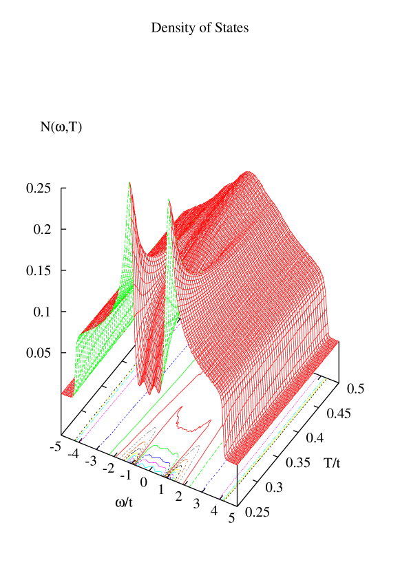
FIG. 4.: A plot of $N(\omega,T)$ versus $\omega$ and $T$. The statistical errors which aren’t shown for clarity are of the order of 0.3%

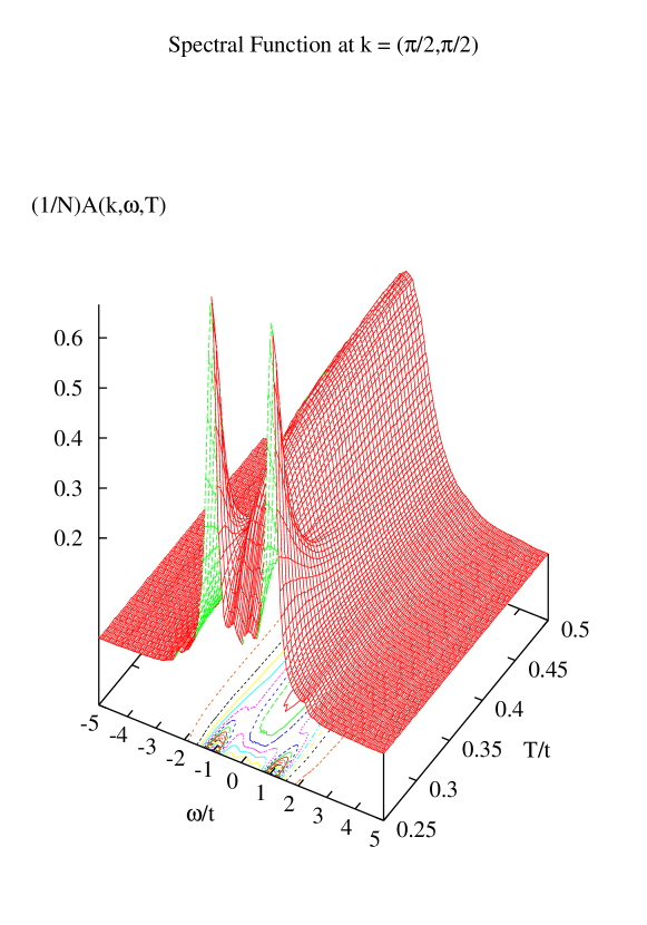
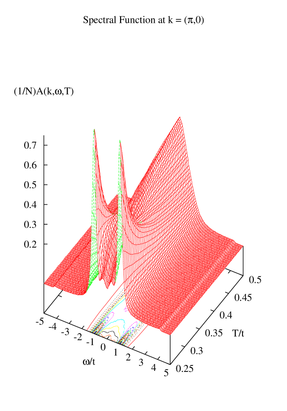
FIG. 5.: a) The single-particle spectral weight $A(k,\omega)$ versus $\omega$ and $T$ for $k=(\pi/2,\pi/2)$ and b) for $k=(\pi,0)$. The statistical errors are of the order of 1%

FIG. 6.: The static spin susceptibility $\chi_{0}(q=0,\omega=0)$ versus $T$ showing the opening of a gap as the temperature is lowered.

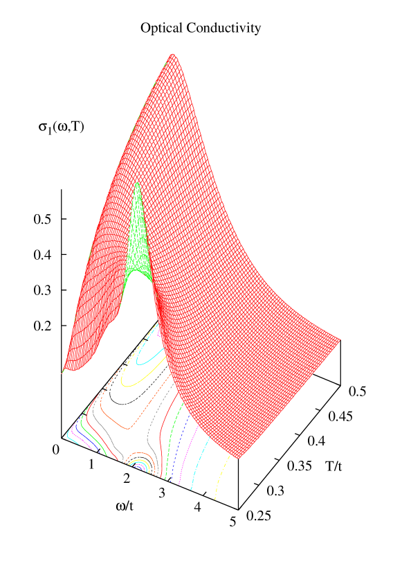
FIG. 7.: Plot of the real part of the optical conductivity $\sigma_{1}(\omega,T)$ versus $\omega$ and $T$ showing the redistribution of spectral weight to higher frequencies as $T_{c}$ is approached. The statistical errors, not shown, are of the order of 0.3%

- [1] A.B. Migdal, Sov. Phys. JETP 7, 996 (1958).
- [2] P.A. Lee, T.M. Rice, and P.W. Anderson, Phys. Rev. Lett. 31, 462 (1973).
- [3] M.V. Sadouskii, Sov. Phys. JETP 39, 845 (1974).
- [4] F. Marsiglio, Phys. Rev. B, 42 2416 (1990).
- [5] A.J. Millis and H. Monien, Phys. Rev. B 61, 12496 (2000).
- [6] R.M. Noack, D.J. Scalapino, and R.T. Scalettar, Phys. Rev. Lett. 66, 778 (1991).
- [7] M. Vekic, R.M. Noack, and S.R. White, Phys. Rev. B 46, 271 (1992).
- [8] H. Monien, Phys. Rev. Lett. 87, 126402 (2001).
- [9] C. Buhler, S. Yunoki, and A. Moreo, Phys. Rev. Lett. 84, 2690 (2000).
- [10] P.E. Lammert and D.S. Rokhsar; cond-mat/0108146.
- [11] T. Eckl, et al.; cond-mat/0110377.
- [12] N.E. Bickers and D.J. Scalapino; cond-mat/0010480.
- [13] F.F. Assaad, cond-mat/0104126.
- [14] R.T. Scalettar, D.J. Scalapino and R.L. Sugar, Phys. Rev. B 34 7911 (1986).
- [15] S. Duane, A.D. Kennedy B.J Pendelton and D. Roweth, Phys. Lett. 195B, 216 (1987).
- [16] M. Creutz, Phys. Rev. D 38 1228 (1988).
- [17] A.M. Ferrenberg and R.H. Swendsen Phys. Rev. Lett. 63, 1195 (1989).
- [18] Note decreases below the “ordering temperature” and is rounded off by finite-size effects.
- [19] Y.M. Vilk and A.-M.S. Tremblay, E urophys. Lett. 33, 159 (1996).
- [20] S. Moukouri et al., Phys. Rev. B 61, 7887 (2000).