Spin Excitations in La₂CuO₄ : Consistent Description by Inclusion of Ring-Exchange

The magnetic properties of La₂CuO₄ have been the subject of many detailed investigations over the last decade. Understanding this undoped parent compound of high temperature superconducting cuprates is a precondition for the many theories which describe metallic cuprates by doping carriers into a layered antiferromagnet. The conventional starting point for undoped cuprates is the two-dimensional (2D) spin-1/2 Heisenberg model with only the nearest-neighbor exchange interaction $J$ [1], which thereby provides the important magnetic energy scale needed as input to theories for the metallic and superconducting properties of doped cuprates. Despite the substantial progress on the theory of the 2D Heisenberg antiferromagnet [2], which includes such physical properties as the temperature dependence of the magnetic correlation length [3, 4], some of the experimental facts for La₂CuO₄ have clearly demonstrated that a complete description of the magnetic excitations requires additional physics not contained in the 2D Heisenberg model with $J$ only. Examples include the asymmetric lineshape of the two-magnon Raman intensity [5] or the infrared optical absorption [6], which have led to proposals that spin-phonon interactions [7], resonant phenomena [8, 9], purely fermionic contributions [10], or cyclic ring-exchange [11, 12, 13] need to be included. In particular, the importance of ring (plaquette) exchange has very recently found direct experimental support from the observed dispersion of the spin-waves along the magnetic Brillouin zone boundary [14].

The 4-spin plaquette ring-exchange interaction $J_{\Box}$ was considered rather early as a possible non-negligible correction to the nearest-neighbor Heisenberg model [15, 16]. This higher-order spin coupling arises naturally in a strong coupling $t/U$ expansion to fourth order for the single band Hubbard model at half-filling [17, 18]. Its quantitative significance was recently demonstrated in high order perturbation expansions [19] and ab initio cluster calculations in realistic three-band Hubbard models for the CuO₂ planes [20]. These derivations of effective spin models for the low-energy magnetic properties of the undoped CuO₂ planes led to the estimate $J_{\Box}/J=0.11$. A linear spin-wave analysis of the spectrum in La₂CuO₄ at 10K in Ref. [14] has deduced a considerably larger value $J_{\Box}/J=0.41$. The necessity for a sizeable $J_{\Box}$ has recently also been conjectured for the spin ladder compound La₂Ca₈Cu₂₄O₄₁[21].

The spin-wave theory and the quasiclassical phase diagram of the frustrated Heisenberg model with ring exchange was investigated in Ref. [22]. However, the quantum and thermal renormalizations have not so far been taken into account in the spin-wave theory. It is well known for the quasi-2D Heisenberg model without the ring-exchange term (see Ref.[23] and references therein) that such renormalizations can substantially change the excitation spectrum of the system. The authors of Ref. [14] considered the simplest renormalization of the spectrum by allowing for an overall quantum renormalization factor, which was obtained for the 2D Heisenberg model with nearest-neighbor exchange within a $1/S$ expansion to order $1/S^{2}$ [24] and by series expansion from the Ising limit [25]. However, in the absence of a consistent analysis of the spin-wave renormalization in the presence of ring-exchange or a next-nearest neighbor coupling, it is not possible to provide an accurate determination of exchange parameters. Indeed, as we show below, the effects of quantum and thermal fluctuations are not simply captured by a single renormalization factor, and a consistent treatment of the spin-wave spectrum with $J_{\Box}\neq$0 to order $1/S$ reveals that the previous early estimate $J$=136meV from high energy neutron scattering [26] or two-magnon Raman scattering [27] requires a correction at least as large as 10%. Also, we show that the recent estimate $J_{\Box}=0.41J$ in Ref. [14] appears to be twice as large as the value calculated by accounting systematically for 1/S renormalizations.

In this paper we consider the corrections to the spin-wave spectrum to first order in $1/S$ for finite $J_{\Box}$ using a self-consistent spin-wave theory [23]. We obtain values of the in-plane and interplane exchange interactions of La₂CuO₄ allowing an accurate fit of the dispersion. We verify that the obtained exchange interactions correctly reproduce the measured values for the spin stiffness and the Néel temperature.

We start from the Heisenberg model with ring-exchange [15, 17, 18]

$$H = {J\over 2}\sum_{i,\delta}{\bf S}_{i}\cdot{\bf S}_{i+\delta}+{J^{\prime}\over 2}\sum_{i,\delta^{\prime}}{\bf S}_{i}\cdot{\bf S}_{i+\delta^{\prime}}+{J^{\prime\prime}\over 2}\sum_{i,\delta^{\prime\prime}}{\bf S}_{i}\cdot{\bf S}_{i+\delta^{\prime\prime}}$$ (1)

$$+ {J_{\perp}\over 2}\sum_{i,\delta_{\perp}}{\bf S}_{i}\cdot{\bf S}_{i+\delta_{\perp}}+J_{\Box}\sum_{\langle ijkl\rangle}\big{[}({\bf S}_{i}\cdot{\bf S}_{j})({\bf S}_{k}\cdot{\bf S}_{l})$$ (2)

$$+ ({\bf S}_{i}\cdot{\bf S}_{l})({\bf S}_{k}\cdot{\bf S}_{j})-({\bf S}_{i}\cdot{\bf S}_{k})({\bf S}_{j}\cdot{\bf S}_{l})\big{]}$$ (3)

where $J$, $J^{\prime}$, and $J^{\prime\prime}$ are the first ($\delta$), second ($\delta^{\prime}$) and third ($\delta^{\prime\prime}$)-nearest-neighbor in-plane exchanges, $\delta_{\perp}$ connects to the nearest-neighbor sites in the adjacent planes with interplane exchange $J_{\perp}$, and $\langle ijkl\rangle$ denotes the four sites of a planar plaquette involved in the ring exchange. We use the Dyson-Maleev representation for the spin operators

$$\left.\begin{array}[]{l}S_{i}^{+}=\sqrt{2S}a_{i}\,,\;S_{i}^{z}=S-a_{i}^{\dagger}a_{i}\\ S_{i}^{-}=\sqrt{2S}(a_{i}^{\dagger}-\displaystyle{1\over 2S}a_{i}^{\dagger}a_{i}^{\dagger}a_{i})\end{array}\right\}\,i\in A\,\,,$$ (4)

$$\left.\begin{array}[]{l}S_{j}^{+}=\sqrt{2S}b_{j}^{\dagger}\,,\;S_{j}^{z}=-S+b_{j}^{\dagger}b_{j}\\ S_{j}^{-}=\sqrt{2S}(b_{j}-\displaystyle{1\over 2S}b_{j}^{\dagger}b_{j}b_{j})\end{array}\right\}\,j\in B\,\,$$ (5)

where $A$ and $B$ denote the magnetic sublattices; $a_{i}^{\dagger},a_{i},$ and $b_{j}^{\dagger},b_{j}$ are Bose operators. After substituting Eqs. (4) and (5) into the Hamiltonian (2), we decouple quartic terms into quadratic ones according to the procedure described in Ref. [23]. Keeping consistently all terms to order $1/S$, we obtain

$$H = S\sum_{i}\sum_{d=\delta,\delta_{\perp}}J_{d}\gamma_{d}(D_{i}^{\dagger}D_{i}+D_{i}^{\dagger}D_{i+d})$$ (8)

$$-S\sum_{i}\sum_{d=\delta^{\prime},\delta^{\prime\prime}}J_{d}\gamma_{d}(D_{i}^{\dagger}D_{i}-D_{i}^{\dagger}D_{i+d})$$

$$-J_{\Box}S^{3}\sum_{i}\sum_{d=\delta,\delta^{\prime}}(\gamma_{0}^{\Box}D_{i}^{\dagger}D_{i}-\gamma_{d}^{\Box}D_{i}^{\dagger}D_{i+d})$$

where $D_{i}=a_{i}$ for $\,i\in A\,$ and $D_{i}=b_{i}^{\dagger}$ for $\,i\in B;\;$also we use the notation $J_{\delta}=J,\;J_{\delta^{\prime}}=J^{\prime}$ etc. The renormalization of the bare exchange parameters due to quantum- and thermal fluctuations is described by the coefficients:

$$\gamma_{d} = \left\{\begin{array}[]{cc}1-[\langle a_{i}^{\dagger}a_{i}\rangle+\langle a_{i}b_{i+d}\rangle]/S,&d=\delta,\delta_{\perp}\\ 1-[\langle a_{i}^{\dagger}a_{i}\rangle-\langle a_{i}^{\dagger}a_{i+d}\rangle]/S,&d=\delta^{\prime},\delta^{\prime\prime}\end{array}\right.\,,$$ (11)

$$\;\gamma_{0}^{\Box} = 1-[3\langle a_{i}^{\dagger}a_{i}\rangle+6\langle a_{i}b_{i+\delta}\rangle+3\langle a_{i}^{\dagger}a_{i+\delta^{\prime}}\rangle]/S\,,$$ (12)

$$\gamma_{\delta}^{\Box} = 1-[3\langle a_{i}^{\dagger}a_{i}\rangle+5\langle a_{i}b_{i+\delta}\rangle+2\langle a_{i}^{\dagger}a_{i+\delta^{\prime}}\rangle]/S\,,$$ (13)

$$\gamma_{\delta^{\prime}}^{\Box} = 1-[3\langle a_{i}^{\dagger}a_{i}\rangle+4\langle a_{i}b_{i+\delta}\rangle+\langle a_{i}^{\dagger}a_{i+\delta^{\prime}}\rangle]/S\,.$$ (14)

Diagonalization of this Hamiltonian yields the spin-wave spectrum

$$E_{{\bf k}} = \sqrt{A_{{\bf k}}^{2}-B_{{\bf k}}^{2}}\,,$$ (15)

$$A_{{\bf k}} = 4S[J\gamma-J^{\prime}\gamma^{\prime}(1-\nu_{{\bf k}}^{\delta^{\prime}})-J_{\Box}S^{2}(\gamma_{0}^{\Box}+\gamma_{\delta^{\prime}}^{\Box}\nu_{{\bf k}}^{\delta^{\prime}})]$$ (17)

$$\ \ \ \ \ \ \ \ -4J^{\prime\prime}S\gamma^{\prime\prime}(1-\nu_{{\bf k}}^{\delta^{\prime\prime}})+2J_{\perp}S\gamma_{\perp}\,,$$

$$B_{{\bf k}} = 4S(J\gamma-J_{\Box}S^{2}\gamma_{\delta}^{\Box})\nu_{{\bf k}}^{\delta}+2J_{\perp}S\gamma_{\perp}\nu_{{\bf k}}^{\delta_{\perp}}\,,$$ (18)

where

$$\nu_{{\bf k}}^{\delta} = (\cos k_{x}+\cos k_{y})/2\;,\;\phantom{22}\nu_{{\bf k}}^{\delta^{\prime}}=\cos k_{x}\cos k_{y}\;,$$ (19)

$$\nu_{{\bf k}}^{\delta^{\prime\prime}} = (\cos 2k_{x}+\cos 2k_{y})/2\;,\;\nu_{{\bf k}}^{\delta_{\perp}}=\cos k_{z}\,,$$ (20)

and $\gamma=\gamma_{\delta}$, $\gamma^{\prime}=\gamma_{\delta^{\prime}}$ etc.; the lattice constants are set to unity. Since the equality $\gamma_{0}^{\Box}=2\gamma_{\delta}^{\Box}-\gamma_{\delta^{\prime}}^{\Box}$ is satisfied, the spectrum given by Eq. (15) is necessarily gapless. It is apparent from this result for the dispersion that the renormalization coefficients $\{\gamma_{d},\gamma^{\Box}_{d}\}$ cannot be combined into a single overall renormalization factor. The averages of the bosonic operators which enter in Eqs. (11) and (14) are

$$\langle a_{i}^{\dagger}a_{i}\rangle = \sum_{{\bf k}}\frac{A_{{\bf k}}}{2E_{{\bf k}}}\coth\frac{E_{{\bf k}}}{2T}-\frac{1}{2}\,,$$ (21)

$$\langle a_{i}^{\dagger}a_{i+d}\rangle = \sum_{{\bf k}}\frac{A_{{\bf k}}\nu_{{\bf k}}^{d}}{2E_{{\bf k}}}\coth\frac{E_{{\bf k}}}{2T}\,,$$ (22)

$$\langle a_{i}b_{i+d}\rangle = -\sum_{{\bf k}}\frac{B_{{\bf k}}\nu_{{\bf k}}^{d}}{2E_{{\bf k}}}\coth\frac{E_{{\bf k}}}{2T}\,.$$ (23)

The expression for the sublattice magnetization reads

$$\overline{S}=S-\langle a_{i}^{\dagger}a_{i}\rangle\,.$$ (24)

As previously discussed for quasi-2D magnets[23], Eqs. (11), (14), and (21) must be solved self-consistently. The spin-wave velocity $c$ is obtained by expanding the dispersion at small wavevector $k=\sqrt{k_{x}^{2}+k_{y}^{2}}$, leading to

$$E_{{\bf k}}\simeq ck\;,\;c=2\sqrt{2}Z_{c}JS\,,$$ (25)

where

$$Z_{c} = (A_{\bf 0}/4JS)^{1/2}\left[\gamma-2(J^{\prime}/J)\gamma^{\prime}-4(J^{\prime\prime}/J)\gamma^{\prime\prime}\right.$$ (27)

$$\ \ \ \ \left.+2(J_{\Box}/J)S^{2}(\gamma_{\delta^{\prime}}^{\Box}-\gamma_{\delta}^{\Box})\right]^{1/2}$$

is the spin-wave velocity renormalization factor. For the spin stiffness we obtain the result

$$\rho_{s} = JS^{2}Z_{\rho}\,,$$ (28)

$$Z_{\rho} = (4J\overline{S}_{0}/A_{\bf 0})Z_{c}^{2}\,.$$ (29)

Given $c$ and $\rho_{s}$, the transverse susceptibility follows immediately as

$$\chi_{\perp}=\rho_{s}/c^{2}=\overline{S}_{0}/(2SA_{\bf 0})=Z_{\chi}/(8J)$$ (30)

where $Z_{\chi}=Z_{\rho}/Z_{c}^{2}$. For $J^{\prime}=J^{\prime\prime}=J_{\Box}=J_{\perp}=0$, i.e. the 2D Heisenberg model with only nearest-neighbor exchange, the self-consistent numerical solution of Eqs. (11) and (21) at zero temperature gives [28, 29, 23] $\gamma=1.158$ and $\overline{S}_{0}=0.303$, which corresponds to $Z_{c}=1.158,\;Z_{\rho}=0.702$, and $Z_{\chi}=0.524$. We note that due to the relations (29) and (30), $Z_{\rho}$ and $Z_{\chi}$ contain partially contributions of order $1/S^{2}$. The above numbers are close to those found for the 2D nearest-neighbor Heisenberg model in a systematic $1/S$ expansion to order $1/S^{2}$: $Z_{c}=1.179,\;Z_{\rho}=0.724$, and $Z_{\chi}=0.514$ [24]. However, we show below, the presence of next-nearest neighbor and plaquette ring-exchange terms substantially alters these numbers.

We use Eqs. (11), (14), and (21) at zero temperature to fit the experimentally determined planar spin-wave dispersion using the data at T=10K from Ref. [14]. To restrict the number of fitting parameters, we suppose $J^{\prime}=J^{\prime\prime}$. This restriction is well justified by the perturbation expansions of the half-filled one- and three-band Hubbard models [17, 18, 19]. The inelastic neutron scattering data together with our fit result along a selected path in the Brillouin zone at $T=10$K are shown in Fig. 1. The best fit is obtained for the following parameter set:

$$J=151.9\,\text{meV},\,\,J^{\prime}=J^{\prime\prime}=0.025J,\,\,J_{\Box}=0.24J.$$ (31)

While the values of $J^{\prime}$ and $J^{\prime\prime}$ are practically indistinguishable from those in Ref.[14] and $J$ in (31) is only 3% larger, our extracted value of $J_{\Box}$ is 50% lower.

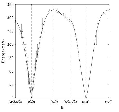
FIG. 1.: Spin-wave dispersion along high symmetry directions in the 2D Brillouin zone. The triangles are the experimental results of Ref. [14] for La₂CuO₄ at 10K. The solid line is the result of a fit to the spin-wave dispersion result (7) leading to the exchange couplings as listed in Eq. (18). The dashed line is the fit of Ref. [14].

For the corresponding groundstate sublattice magnetization $\overline{S}_{0}$ and for the renormalization parameters $\{\gamma_{d},\gamma_{d}^{\Box}\}$ we obtain

$$\overline{S}_{0}=0.319,\;\gamma\phantom{\Box} = 1.158,\;\gamma^{\prime}=0.909,\;\gamma^{\prime\prime}=0.852\,,$$ (32)

$$\gamma_{0}^{\Box} = 2.220,\;\gamma_{\delta}^{\Box}=1.971,\;\gamma_{\delta^{\prime}}^{\Box}=1.721\,.$$ (33)

In our notation, the spectrum used in Ref. [14] corresponds to equal renormalization factors: $\gamma=\gamma^{\prime}=\gamma^{\prime\prime}=\gamma_{i}^{\Box}\simeq 1.18$; the parameter values obtained with this spectrum were $J^{\prime}/J=J^{\prime\prime}/J=0.020$, and $J_{\Box}/J=0.41$. However, some of the $\gamma$-coefficients show a remarkable deviation from the value 1.18 found for the 2D system with nearest-neighbor exchange only [24]. In particular the renormalization coefficients $\{\gamma_{d}^{\Box}\}$ for the ring-exchange deviate very strongly. We emphasize again, although some fitting parameters are very similar to [14], it is the self-consitently renormalized parameters $\{\gamma_{d},\gamma_{d}^{\Box}\}$ which allow us to obtain an accurate and reliable set of bare superexchange couplings.

In the self-consistent spin-wave theory presented here the in-plane magnon spectrum varies only weakly with temperature at $T\ll J$. Although the spectrum changes qualitatively in the same way as found experimentally, it accounts only for a few per cent of the observed changes in the zone boundary dispersion of the data at $T=295K$ in Ref. [14].

From the parameter values obtained above we deduce the spin stiffness, the spin-wave velocity, and the transverse susceptibility: $\rho_{s}=23.8$ meV, $c=206$ meV and $\chi_{\perp}=4.8\times 10^{-5}$K${}^{-1}.$ The corresponding values of the renormalization factors as calculated from Eqs. (27), (29), and (30) are $Z_{c}=0.96$, $Z_{\rho}=0.63$ and $Z_{\chi}=0.68$. These values differ substantially from those for the 2D nearest-neighbor Heisenberg model. We note that our value for the spin stiffness is in very good agreement with the earlier estimate [30] $\rho_{s}=23.9$meV found from fitting the spin-spin correlation length $\xi(T)$ at $T>T_{N}$ to the non-linear $\sigma$-model result [2] with the correct preexponential factor[3]. This agreement strongly supports the validity of the self-consistent renormalized spin-wave theory.

As discussed in Refs. [23, 31], it is difficult to fit the value $J_{\perp}$ from measurements of the out-of-plane spin-wave spectrum. Instead, we use an alternative procedure and fit the temperature dependence of the sublattice magnetization at temperatures $T<T_{N}/2$ where the above theory is reliable (cf. Ref.[23] and references therein) employing the exchange parameters listed in (31). In this way we obtain $J_{\perp}/J=1.0\times 10^{-3}$ and $\gamma_{\perp}/\gamma=5.67\times 10^{-4}$ which practically coincides with the previous estimate in Refs. [23, 31].

As another test of the above results, we also calculate the Néel temperature for the obtained exchange parameter values. On the basis of a renormalization-group approach and a $1/N$ expansion in the $O(N)$ quantum nonlinear $\sigma$-model, the result for the Néel temperature of a quasi-2D isotropic Heisenberg antiferromagnet has the form [23, 31]

$$T_{N}=4\pi\rho_{s}\left[\ln\frac{T_{N}^{2}}{c^{2}\alpha_{r}}+3\ln\frac{4\pi\rho_{s}}{T_{N}}-0.0660\right]^{-1}$$ (34)

where $\alpha_{r}=(\gamma_{\perp}/\gamma)_{T=0}$, and $c$ and $\rho_{s}$ are the respective groundstate spin-wave velocity and spin stiffness given by Eqs. (28) and (25). With the above parameter values (31) we obtain $T_{N}=328K$, in almost perfect agreement with the experimental value $T_{N}=325K$ [30].

In conclusion, we have considered the renormalization of the spin-wave spectrum to order $1/S$ for the Heisenberg antiferromagnet in the presence of plaquette ring-exchange. The results allow for an accurate fit of the magnon dispersion in La₂CuO₄ and a consistent determination of the exchange coupling parameters for this material. As an independent check of the parameter set, the spin stiffness and the Néel temperature are correctly reproduced. With $J=151.9$meV the obtained value for the bare ring-exchange coupling $J_{\Box}/J=0.24$ in La₂CuO₄ is significant although due to its 4-spin coupling the ring-exchange term in the Hamiltonian will be reduced by a factor $S^{2}$ with respect to the $J$ term. The magnitude of $J_{\Box}$ suggests that for hole doped cuprates ring-exchange might be relevant, too, and we may postulate that it is connected to recent proposals of staggered circulating currents in underdoped materials [32, 33]. The role of ring-exchange for the spectral lineshape of the $B_{1g}$ shift in Raman experiments and for infrared absorption remains to be reexplored and contrasted to the recent proposal of a purely fermionic origin of spectral weight at higher energies [10].

It is a pleasure to thank B. Normand and T. Kopp for useful discussions. We are indebted to G. Aeppli for sending us experimental data for the spin wave dispersion. We acknowledge support through Sonderforschungsbereich 484 of the Deutsche Forschungsgemeinschaft.

REFERENCES

[1] E. Manousakis, Rev. Mod. Phys. 63, 1 (1991).
[2] S. Chakravarty, B. I. Halperin, and D. R. Nelson,
Phys. Rev. B 39, 2344 (1989).
[3] P. Hasenfratz and F. Niedermayer, Phys. Lett. B 268, 231 (1991).
[4] P. Carretta, T. Ciabattoni, A. Cuccoli, E. Mognaschi, A.
Rigamonti, V. Tognetti, and P. Verrucchi, Phys. Rev. Lett. 84, 366
(2000).
[5] K. B. Lyons, P. E. Sulewski, P. A. Fleury, H. L. Carter, A. S.
Cooper, and G. P. Espinosa, Phys. Rev. B 39, 9693 (1989); S. Sugai et
al., ibid. 42, 1045 (1990).
[6] J. D. Perkins, J. M. Graybeal, M. A. Kastner, R. J.
Birgeneau, J. P. Falck, and M. Greven, Phys. Rev. Lett. 71, 1621 (1993).
[7] F. Nori, R. Merlin, S. Haas, A. W. Sandvik, and E. Dagotto,
Phys. Rev. Lett. 75, 553 (1995).
[8] A. Chubukov and D. Frenkel, Phys. Rev. Lett. 74, 3057 (1995).
[9] F. Schönfeld, A. P. Kampf, and E. Müller-Hartmann,
Z. Phys. B 102, 25 (1997).
[10] C.-M. Ho, V. N. Muthukumar, M. Ogata, and P. W. Anderson, Phys.
Rev. Lett. 86, 1626 (2001).
[11] Y. Honda, Y. Kuramoto, and T. Watanabe, Phys. Rev. B 47,
11329 (1993).
[12] J. Eroles, C. D. Batista, S. B. Bacci, and E. R. Gagliano,
Phys. Rev. B 59, 1468 (1999).
[13] J. Lorenzana, J. Eroles, and S. Sorella, Phys. Rev.
Lett. 83, 5122 (1999).
[14] R. Coldea, S. M. Hayden, G. Aeppli, T. G. Perring, C. D.
Frost, T. E. Mason, S.-W. Cheong, and Z. Fisk, Phys. Rev. Lett. 86,
5377 (2001).
[15] M. Roger and J. M. Delrieu, Phys. Rev. B 39, 2299
(1989).
[16] H. J. Schmidt and Y. Kuramoto, Physica (Amsterdam) 167C, 263 (1990).
[17] M. Takahashi, J. Phys. C: Solid State Phys. 10,
1289 (1977).
[18] A. H. MacDonald, S. M. Girvin, and D. Yoshioka, Phys.
Rev. B 41, 2565 (1990); Phys. Rev. B 37, 9753 (1988).
[19] E. Müller-Hartmann and A. Reischl, cond-mat/0105392
[20] C. J. Calzado and J.-P. Malrieu, cond-mat/0010259
[21] M. Matsuda, K. Katsumata, R. S. Eccleston, S. Brehmer,
and H.-J. Mikeska, Phys. Rev. B 62, 8903 (2000).
[22] A. Chubukov, E. Gagliano, and C. Balseiro, Phys. Rev. B
45, 7889 (1992).
[23] V. Yu. Irkhin, A. A. Katanin, and M. I. Katsnelson, Phys.
Lett. A 157 (1991); Phys. Rev. B 60, 1082 (1999).
[24] C. M. Canali and S. M. Girvin, Phys. Rev. B 45, 7127
(1992); C. M. Canali, S. M. Girvin, and M. Wallin, ibid.45, 10131
(1992); I. Igarashi, ibid.46, 10763 (1992).
[25] R. R. P. Singh, Phys. Rev. B40, 7247 (1989);
R. R. P. Singh and M. P. Gelfand, ibid. 52, R15695 (1995).
[26] S. M. Hayden, G. Aeppli, R. Osborn, A. D. Taylor, T. G.
Perring, S.-W. Cheong, and Z. Fisk, Phys. Rev. Lett. 67, 3622 (1991).
[27] R. R. P. Singh, P. A. Fleury, K. B. Lyons, and P. E.
Sulewski, Phys. Rev. Lett. 62, 2736 (1989).
[28] M. Takahashi, Phys. Rev. B 40, 2494 (1989).
[29] D. Yoshioka, J. Phys. Soc. Jpn. 58, 3733 (1989).
[30] B. Keimer, A. Aharony, A. Auerbach, R. J. Birgeneau, A.
Cassanho, Y. Endoh, R. W. Erwin, M.A. Kastner, and G. Shirane, Phys. Rev. B
45, 7430 (1992); Phys. Rev. B 46, 14034 (1992).
[31] V. Yu. Irkhin and A. A. Katanin, Phys. Rev. B 55,
12318 (1997); ibid. 57, 379 (1998).
[32] C. M. Varma, Phys. Rev. B 55, 14554 (1997), Phys. Rev.
Lett. 83, 3538 (1999).
[33] S. Chakravarty, R. B. Laughlin, D. K. Morr, and C. Nayak,
Phys. Rev. B 63, 094503 (2001).