Localized defects in a cellular automaton model for traffic flow with phase separation

Abstract

We study the impact of a localized defect in a cellular automaton model for traffic flow which exhibits metastable states and phase separation. The defect is implemented by locally limiting the maximal possible flow through an increase of the deceleration probability. Depending on the magnitude of the defect three phases can be identified in the system. One of these phases shows the characteristics of stop-and-go traffic which can not be found in the model without lattice defect. Thus our results provide evidence that even in a model with strong phase separation stop-and-go traffic can occur if local defects exist. From a physical point of view the model describes the competition between two mechanisms of phase separation.

, , , , and

1 Introduction

Nowadays mobility, mostly realized by means of vehicular traffic, is an integral part of any modern society. Unfortunately, the capacity of the existing road networks is often exceeded in densely populated areas and the possibilities for a further expansion are very limited. Therefore experimental and theoretical investigations of traffic flow have been the focus of extensive research during the past decades with the aim to optimize the usage of existing capacities.

In many cases it seems as if the occurrence of traffic states with high density like jammed or synchronized traffic can be linked to external influences, e.g., on- and off-ramps, bottlenecks, lane reductions or road works (see [1, 2, 3, 4, 5, 6, 7, 8]). Such local perturbations can act as a seed for the formation of jammed traffic states which finally spread through large parts of the network. Hence local defects can have a crucial impact on the overall network performance. A proper understanding of the interactions between local defects and model dynamics and its consequences is indispensable for realistic large scale computer simulations.

In recent years various theoretical approaches for the description of traffic flow have been suggested (for reviews, see e.g, [9, 10, 11, 12, 13]) which can be divided into macroscopic and microscopic models. Today one of the main interests in applications to real traffic is to perform real-time simulations of large networks with access to individual vehicles. In contrast to macroscopic models, microscopic models provide information about the behavior of individual vehicles. Due to their simplicity cellular automata (CA) have become quite popular in the field of microscopic traffic modeling. The first CA model for traffic flow with the ability to reproduce the basic phenomena encountered in real traffic, e.g., the occurrence of phantom traffic jams, was proposed by Nagel and Schreckenberg (NaSch) [14]. However, the NaSch model can by far not explain all empirical results like the velocity of jam fronts or the reduced outflow from jams leading to metastable states. Therefore modifications have been suggested to obtain a description of the traffic dynamics on a more detailed level. In this paper we focus our investigations on the NaSch model with velocity-dependent randomization (VDR model) [15] which exhibits metastable states and shows phase separation into free flow and wide jams. Because of the strong phase separation it turns out that the VDR model is an interesting candidate for investigating the influence of external perturbations on the internal model dynamics. Due to the fact that only wide jams appear in an undisturbed system, any additional high density patterns induced by external forces can be identified easily.

The impact of defects in the NaSch model (and related models, e.g., the asymmetric simple exclusion process (ASEP)) is by now well understood. Basically two types of defects can be distinguished which can be characterized as particlewise and sitewise disorder, respectively [16]. In a model where a finite number (in the thermodynamic limit) of particles (vehicles) or sites has different properties from the rest these are usually called defects. In the first case, corresponding to a limiting case of particlewise disorder [17, 18, 19], the defect particles may have a smaller maximal velocity. Such defects are not localized in space in contrast to those corresponding to sitewise disorder where in a localized region certain parameters of the model take different values, e.g., by imposing a speed limit or increasing the deceleration probabilities [20, 21, 22, 23, 24, 25, 26, 27].

In both cases a parameter regime exists where the global behavior of the system is controlled by the defect which acts as a bottleneck. Generically it induces phase separation into a high and a low density region separated by a sharp discontinuity (“shock”). In the case of particlewise disorder with one slow car (and no overtaking) the faster cars tend to pile up behind the slow one. This behavior has certain similarities with Bose-Einstein condensation [17]. For a spatially localized defect one also finds a separation into a high and a low density regime, but with the high density region pinned to the defect. This behavior has been found in a variety of models and for different defect realizations. However, none of the models investigated so far exhibits phase separation through the existence of high-flow metastable states which is an important ingredient for any realistic traffic model.

In the present paper we investigate the influence of a localized defect on a traffic model exhibiting metastable states. This allows to study the interplay between two very different mechanisms for phase separation, i.e., one driven by the dynamics of the particles and one driven by the defect. Our investigations of the VDR model reveal the occurrence of three different phases whereby one of them shows the characteristics of stop-and-go traffic. Note, that these phases can not be obtained in the model without lattice defect. Moreover, concerning the question whether certain jam patterns found in real traffic are induced by local defects or due to the internal behavior of the drivers our findings allow a deeper insight into possible methods of modeling such traffic states. In the VDR model individual driving behavior is realized by a simple stochastic parameter. For the purpose of keeping the set of model parameters manageable we implemented the local defect in our investigations simply by increasing this stochastic noise in a specific part of the system.

2 Definition of the Model

Figure 1: Schematic representation of the local defect. The defect itself is placed at a fixed position on a periodic one lane street. Its width is chosen to $v_{\text{max}}$ cells.

In the spirit of modeling complex phenomena in statistical physics one is interested in keeping the model as simple as possible. Obviously, the modeling of traffic flow in the language of cellular automata (CA) always implies an extreme simplification of real world conditions. Hence space, speed, acceleration, and even time are treated as discrete variables and the motion is realized in the ideal case by a minimal set of local rules. In this manner we tried to find a straightforward representation for local defects on a one-lane street in the VDR model. Since the model contains a stochastic parameter which is needed to implement various phenomena found in real traffic, e.g., spontaneous jam formation, reduced outflow from a jam, it seems obvious to implement a local defect by increasing this parameter in a limited area. As mentioned before, other types of localized defects have been studied in the NaSch model and related models, e.g., reducing the maximal velocity of the cars locally. Introducing a locally lower speed limit in the VDR model should have the same effect as the enhanced deceleration probability since one expects also phase separation into high and low density regions in a certain regime of the global density. However, the microscopic details of the states can be different for the various defect types.

For the sake of completeness, we will briefly recall the definition of the VDR model [15]. The road is divided into cells of length $7.5m$. Each cell can either be empty or occupied by just one car. The speed of each vehicle can take one of the $v_{\text{max}}+1$ allowed integer values $v=0,1,...,v_{\text{max}}$. The state of the road at time $t+1$ can be obtained from that at time-step $t$ by applying the following rules to all cars at the same time (parallel dynamics):

• Step 1: Acceleration:
  $v_{n}\rightarrow\min(v_{n}+1,v_{\text{max}})$
  

• Step 2: Braking:
  $v_{n}\rightarrow\min(v_{n},d_{n}-1)$
  

• Step 3: Randomization: with probability $p=p(v)$
  $v_{n}\rightarrow\max(v_{n}-1,0)$
  

• Step 4: Driving:
  $x_{n}\rightarrow x_{n}+v_{n}$

Here $d_{n}=x_{n+1}-x_{n}$ denotes the distance (‘headway’) to the next car ahead. One time-step corresponds to approximately $1s$ in real time. Note, that the fluctuation parameter $p=p(v)$ depends on the velocity whereas it is constant in the NaSch model. This parameter has to be determined before the acceleration in “step 1”. For simplicity we study the so called slow-to-start case with two stochastic parameters:

$$p(v)=\left\{\begin{array}[]{ccc}p_{0}&\qquad\text{for}&v=0,\\ p&\qquad\text{for}&v>0.\end{array}\right.$$ (1)

Thereby, $p_{0}$ controls the fluctuations of cars a rest, i.e., determines the velocity of a jam, and $p$ controls the velocity fluctuations of moving cars. In the case $p_{0}\gg p$ the model shows the expected features: phase separation and metastable states. It is interesting that an alternative choice of $p(v)$, e.g., $p_{0}\ll p$ leads to a completely different behavior. Note that for $p_{0}=p$ the original NaSch model is recovered. If not stated otherwise, $p_{0}$ is set to $0.5$ and $p$ to $0.01$ throughout this paper. These parameter values yield a good agreement with empirical results (see [15, 29] for further details).

As mentioned before the local defect is implemented by increasing the stochastic noise parameter $p(v)$ in a limited area of the system. Various implementations of a local defect are possible, but here we want to keep the set of parameters as small as possible. The length of the defect is chosen to $L_{d}$ cells and the stochastic noise $p(v)$ is replaced by a defect noise $p_{d}$. The defect length $L_{d}$ itself is set to $L_{d}=v_{\text{max}}$ to ensure that each car will participate at least once in an update with the enhanced breaking probability $p_{d}$. Note, that this also implies that slow vehicles underly a stronger influence. They need more than one timestep to cross the defect region and thus the defect deceleration rule has to be applied more often than for fast cars which can cross the defect in one timestep.

Given that the stochastic noise in the VDR model depends on the velocity of vehicles, the choice of the stochastic parameter inside the defect must be seen with respect to this. Our strategy is to choose the stochastic noise in a way that it is maximal. In detail one gets the following equation:

$$p(x,v)=\left\{\begin{array}[]{ccc}\max(p(v),p_{d})&\text{for}&x\in D,\\ p(v)&\text{for}&x\notin D,\end{array}\right.$$ (2)

with $D=\{x|x_{f}\leq x\leq x_{l}\}$ denoting the cells forming the defect. Here $x_{f}$ is the first cell of the defect and $x_{l}$ the last one. In Fig. 1 a schematic representation of the local defect with all its parameters is depicted. Obviously, the defect width as well as $p_{d}$ control the strength of the defect. For the sake of simplicity, we keep the width of the defect fixed and chose $p_{d}$ as control parameter. The influence of different spatial extensions of the defect is studied in [27].

3 Numerical results

 

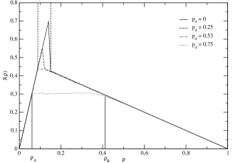
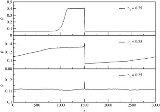
Figure 2: Left: Typical fundamental diagram of the VDR model with a lattice defect. The different defect noise parameters $p_{d}$ cover the occurring phases. The remaining model parameters are $L=3000$, $v_{\text{max}}=5$, $p_{0}=0.5$ and $p=0.01$. Right: Density profiles of the analyzed system for density $\rho=\frac{1}{9}$. Starting from bottom to top: The case $p_{d}=0.25$ corresponds to the VDR phase. Only a small peak at the defect is observable representing the interactions between the defect and the vehicles. For an intermediate defect noise, here $p_{d}=0.53$, the density profile is almost linear due to the different lifetimes of the small jams emerging at the defect. In the high defect noise case with $p_{d}=0.75$ (stop-and-go phase) the system self-organizes into macroscopic high and low density regimes similar to the NaSch model with defect.

In this section we discuss the impact of the local defect scenario introduced in the previous section on the basis of numerical results. We use the stochastic noise $p_{d}$ inside the local area belonging to the defect as control parameter. The other parameters of the model are kept fixed ($L=3000,v_{\text{max}}=5,p_{0}=0.5,p=0.01$). Starting from low $p_{d}$ three different phases can be distinguished in the system.

At this point it should be mentioned that the fundamental diagram of the VDR model shows three different regimes with respect to the density (Fig. 2, $p_{d}=0$). Up to a certain density $\rho_{1}$ the system is in a free flow state, i.e., no jams exist. Above the density $\rho_{2}$ the system resides in the so called jammed state. This state is characterized by wide phase separated jams and free flowing vehicles. However, the most interesting regime lies between the two densities $\rho_{1}$ and $\rho_{2}$ where the system can be in two different states. One is a metastable homogeneous state with an extremely long lifetime and a high flow where jams can appear due to internal fluctuations. The other one is a phase separated state with wide jams which can be reached through the decay of the homogeneous state or directly owing to the initial conditions. A typical fundamental diagram for the considered system is plotted in Fig. 2 for different $p_{d}$. The case $p_{d}=0$ corresponds to the undisturbed VDR model. The metastable branch with high flow between $\rho_{1}$ and $\rho_{2}$ can clearly be identified.

3.1 Small defect noise: $p_{d}\ll p$

For a low stochastic noise inside the defect $p_{d}\ll 1$, the influence on the overall dynamics of the system is negligible. The only exception is the lifetime of the metastable states occurring in the VDR model which is decreasing strongly. The reason is that the metastable states of the VDR model are very sensitive in regard to perturbations. In [30] an analytical expression for the sensitivity, i.e., the probability that a perturbation of finite magnitude destroys the metastable state, is presented. As one can see in Fig. 2 (left), the maximal possible flow of the metastable branch is reduced extremely for $p_{d}=0.25$ which is chosen as a typical value for a small defect noise. Obviously other values for $p_{d}$ lead to different lifetimes. However, the term “small noise” should not be related to the lifetimes of the metastable states but rather to the impact on the systems dynamics after the transition from a metastable high-flow state to a jammed state. Thus a defect noise is “small” if the jammed state of the system is nearly unaffected by it. This phase will be denoted as the VDR phase since it matches with the jammed state of the VDR model. It is characterized by a wide jam, which moves backwards and is able to pass the defect area uninfluenced, and free flowing vehicles. The distribution of headways in the latter is determined completely by the outflow from the jam. The distance between the free flowing vehicles is large enough to absorb additional velocity fluctuations in the area of the defect without the emergence of new jams. In Fig. 2 (right) the density profile of the considered system is shown for various $p_{d}$. The VDR phase shows a constant density profile with a small peak in the area of the defect. This peak is created by the additional velocity fluctuations which lead to increased travel times. Besides this peak there is no markable difference to the jammed state of the VDR model.

3.2 Large defect noise: $p_{d}\gg p$

As expected, large defect noises $p_{d}$ have a significant influence on the flow of the system. Three different density regimes can be distinguished corresponding to the ones found in the NaSch model under the same circumstances [26]. At low densities the average distance between the vehicles is large enough to compensate velocity fluctuations induced by the defect. Similarly for high densities the system is dominated by jams whose movement is nearly unhindered. Thus the fundamental diagram in Fig. 2 coincides for these two density regimes with the one of the undisturbed model. However, the most interesting density regime is situated in the middle of the fundamental diagram and can be identified by a plateau. This plateau is formed since the capacity of the defect limits the global flow in the system. It can not exceed the maximal flow $J_{\text{def}}$ through the defect which therefore cuts off the fundamental diagram at $J_{\text{def}}$ and leads to the formation of the plateau. The plateau value decreases almost linearly with an increasing defect noise. As one can see in the corresponding space-time plot Fig. 3 (left), a considerable amount of vehicles is gathered at the defect forming a high density region. The width of this high density region itself grows linearly with increasing density as long as densities corresponding to the plateau are considered $\rho_{A}<\rho<\rho_{E}$ (for a detailed analysis see [27]). Fig. 2 (right) shows the density profile for a density within the plateau region. The system self-organizes into a macroscopic high density region pinned at the defect and a low density region determined by the capacity of the defect. So far the macroscopic properties are comparable to results obtained by the NaSch model with a local defect [26]. However, a look at the microscopic structure of the high density region reveals some interesting differences. In contrast to the NaSch model, where the high density region at the defect consists of a compact congested region, the high density region in the VDR model is characterized by small compact jams which are separated by free flow regimes (see Fig. 3 (left)). The term “small compact jams” means that the jams at the defect are significantly smaller than the width of the high density region. This specific jam pattern shows some similarities with stop-and-go traffic and will therefore be called stop-and-go phase. However, the correspondence to real world traffic patterns should be viewed in a qualitatively sense here. The stop and go phase is characterized by a relatively large jammed region (high density) consisting of jams alternating with free flow sections. Here it is important to keep in mind that the high density region is not distinguishable from the one occurring in the NaSch model if considering only macroscopic quantities. The microscopic structure shows a new high density state which cannot be found in the NaSch model. Therefore it will be analyzed in a future work in more detail. Moreover, it must be stressed that the local defect is an essential ingredient for the occurrence of stop-and-go traffic in the VDR model (an undisturbed system shows only free flow or one single wide jam) while in the NaSch model jams of various sizes can occur even in an undisturbed system [12]. One has to take into account that the so called slow-to-start case $p_{0}\gg p$ of the VDR model is considered here, which leads to the occurrence of compact wide jams. In general for parameter combinations with $p<p_{0}$ even in the VDR model stop-and-go traffic can be found. Thus the absence of this specific traffic state is not a limitation of the model, but rather due to the special choice of fluctuation parameters. However, we have focussed on the slow-to-start case $p_{0}\gg p$ here since we are interested in the effects of the competition between the bulk and the defect dynamics.

  

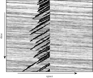
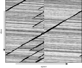
Figure 3: Space-time plot of the analyzed system for a density of $\rho=\frac{1}{8}$. Left: The high defect noise ($p_{d}=0.75$) state is characterized by a high density region consisting of small compact jams which are separated by small free flow regions. Whereas this jam pattern is pinned at the defect and shows some similarities to stop-and-go traffic. Right: For an intermediate defect noise $p_{d}=0.53$ a mixture of a wide jam moving nearly undisturbed through the system and small jams which are formed at the defect is observable. The different lifetimes of the small jams lead to an approximately linear density profile (see Fig. 2 right).

3.3 Transition regime: $p_{d}\approx p$

In the following we focus our investigations on intermediate values of the defect noise parameter $p_{d}$. The space-time plot in Fig. 3 (right) exhibits the microscopic structure of the stationary state for this parameter region. In particular a wide jam moves backwards through the system and additionally some small jams are formed at the defect which have a limited lifetime. Note, that as in the case of large and small $p_{d}$ the defect has almost no influence on the dynamics of the system for low and high densities. Therefore we will focus on intermediate densities to demonstrate effects caused by the additional localized noise parameter $p_{d}$. As one can see in Fig. 2 the described mixture of a wide jam and some small ones cannot be identified easily in the fundamental diagram. The flow is almost identical to that in the model without defect except for the missing metastable branch. This is rather different from the case of large $p_{d}$ where a plateau is formed in the fundamental diagram. This suggests that for an intermediate $p_{d}$ the capacity of the defect is close to the maximum possible flow in the system. Furthermore, taking a look at the density profile for a corresponding intermediate defect noise (respectively $p_{d}=0.53$) another difference to the large $p_{d}$ case is observable. For a large $p_{d}$ the system self-organizes into a macroscopic high density region pinned at the defect and a low density region. In contrast, for intermediate values of $p_{d}$ the density profile decreases approximately linear in upstream direction at the defect. This behavior can be traced back to the different lifetimes of the small compact jams. The dynamics of such a small jam can be described analytically by random walk arguments as shown in [30].

This marks an important difference to the behavior of the NaSch model with a defect. Here a comparable state does not exist. This finding is also interesting for the interpretation of empirical results. Traffic states consisting of wide jams passing a localized region with a flow comparable to free flow and small mean velocity (these states are often denoted as synchronized traffic) are observable in real traffic [31, 32]. However, the system state for intermediate $p_{d}$ has to be interpreted as a crossover phase. For small $p_{d}$ it was shown that only one single wide jam moves undisturbed through the system while for a high $p_{d}$ no single wide jam can exist. In contrast a region with many small jams is formed at the defect (stop-and-go traffic). Starting from small $p_{d}$ without any small jams in the system one can observe the occurrence of small jams at the defect with an increasing frequency if increasing the defect noise $p_{d}$. Further increasing the defect noise finally leads to the complete dissolving of the large jam. Now the system shows only stop-and-go traffic in the vicinity of the defect. To identify this transition between the crossover phase containing one large and various small jams and the stop-and-go phase (large $p_{d}$) we investigate the autocorrelation function in the following.

 

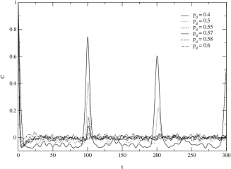
Figure 4: Left: The autocorrelation function shows peaks at a regular distance representing the wide backward moving jam in the system. The height of the peaks decreases with increasing $p_{d}$ until the peak vanish completely because the transition to the stop and go phase occur. Right: Plot of the maximum of the first peak as function of the defect noise $p_{d}$. The vanishing point of the peak is determined through an extrapolation is plotted using an exponential fit function.

The density autocorrelation function $\mathcal{C}$ which is defined as

$$\mathcal{C}=\frac{1}{T}\frac{\sum_{\tau=1}^{T}\rho_{l_{\tau}}\rho_{l_{\tau+\Delta T}}-\frac{1}{T}\sum_{\tau=1}^{T}\rho_{l_{\tau}}\sum_{\tau=1}^{T}\rho_{l_{\tau+\Delta T}}}{\langle\rho^{2}\rangle-\langle\rho\rangle^{2}},$$ (3)

with the local density $\rho_{l}$ of a site at position $x_{n}$,

$$\rho_{l}(i)=\frac{1}{T}\sum_{t=1}^{T}\frac{1}{v_{n}}\;\;\qquad\quad\mbox{with}\;(x_{n}-v_{n})<i\;\;\mbox{and}\;\;x_{n}>i,$$ (4)

can be used to distinguish between the phase with stop-and-go traffic (pinned at the defect) and the intermediate $p_{d}$ region where crossover behavior is observed. The autocorrelation function is able to detect periodically moving structures, i.e., large moving jams. For small $p_{d}$ (VDR phase) as well as for intermediate $p_{d}$ (crossover phase) the system is characterized by a wide jam which recurs periodically due to the periodic boundary conditions. The autocorrelation function is capable to specify the point at which this wide jam vanishes, i.e., the transition point to the pinned stop-and-go phase. Remember, that in the case of crossover behavior additionally small jams are formed at the defect. However, these small jams do not affect the autocorrelation function at all since their lifetime is not large enough to move throughout the whole system.

In Fig. 4 (left) the density autocorrelation function is plotted against the time lag $\Delta T$. The curve shows peaks with a regular distance which represent the wide jam moving backwards through the periodic system. It can clearly be seen that the height of the peaks decreases with increasing $p_{d}$ until they finally vanish completely, i.e., the wide jam dissolves and the transition to the pinned phase occurs. Besides, the autocorrelation function can be used to determine the velocity of jams in the model which is given by the distance between the peaks and the corresponding length of the system (see [33] for further details).

In order to determine the transition point we concentrate on the absolute value of the first peak. This peak value is plotted as function of the defect noise parameter $p_{d}$ (Fig. 4). To obtain the transition point the curve is extrapolated to zero, i.e., vanishing peak values. This is done using the fit function $f(x)=1-\alpha e^{-\beta x}$ which reproduces the shape of the curve quite accurately. In Fig. 4 (right) the values of the first peak are shown with the corresponding exponential fit for the global density $\rho=1/6$. For these parameters we get the best fit with $\alpha=0.01$ and $\beta=-7.9$. The crossing through zero is obtained for a defect noise of $p_{d}=0.57$. For further results concerning the transition to the pinned phase see [27].

3.4 Relevance for systems with ramps

It has been realized recently [34, 35, 36, 8] that inhomogeneities like on- and off-ramps play an important role in real traffic. They might be the origin of a variety of different traffic states observed empirically. For the NaSch model it has been found in [37] that the effects of ramps are very similar to those of localized defects. The presence of an on-ramp leads to a local increase of the density and a restriction of the maximal possible flow. The fundamental diagram shows a plateau and the plateau value is determined by the inflow from the ramp. Also the microscopic structure of the states in systems with defects and ramps is very similar.

For the case of the VDR model with ramps we also find for small ramp flows a phase similar to the VDR phase in defect systems. However, the width of the jam varies close to the on- and off-ramp where it becomes larger or smaller, respectively. For large ramp flows a phase similar to the stop-and-go phase in the defect model is realized. It is characterized by a high density region of stop-and-go traffic pinned to the ramp. Furthermore a transition region can be identified where a large moving jam coexists with smaller jams which are pinned at the ramps.

This shows that also the VDR models with defects and ramps exhibit a rather similar behavior. However, there are subtle differences which are discussed in [27].

4 Summary and discussion

We have analyzed the impact of a local lattice defect in the VDR model. An important aspect is the competition between two mechanisms of phase separation. The dynamics of the VDR model leads to a phase separation at high densities into a large moving jam and a free flow region. In contrast, a localized defect triggers the formation of a high density region pinned at the defect. From a practical point of view our aim was to obtain a deeper insight into the formation of jam patterns due to topological peculiarities. The local defect itself was implemented by increasing the stochastic noise of vehicles within a certain area. Three different system states (phases) can be observed as the defect noise $p_{d}$ is varied. Small defect noises $p_{d}$ reduce the lifetimes of the metastable states in the VDR model which show a strong sensitivity to disturbances. The vehicles in the jammed state of the system, consisting of a single wide jam and free flow, can pass nearly undisturbed through the defect. We denoted this phase as VDR phase since there is almost no difference to the jammed state of the VDR model without defect. In contrast to the low $p_{d}$ case, for a large $p_{d}$ a pinned high density region is formed at the defect limiting the overall system flow. The microscopic structure of this high density region reveals the occurrence of small compact jams which are separated by small free flow regions. This phase is called stop-and-go phase since the jam pattern shows strong similarities to stop-and-go traffic. An important point is that stop-and-go traffic cannot be found in the VDR model without a lattice defect. Furthermore, we found crossover behavior for an intermediate defect noise $p_{d}$. Here a wide jam moves backwards through the system. Additionally small jams are formed at the defect which have a limited lifetime. In order to determine the transition point between this crossover phase, containing one wide jam and various small jams, and the stop-and-go phase, where no wide jam can be found, we investigated the density autocorrelation function.

To conclude, the results presented here are of practical relevance for traffic flow simulations using simple stochastic CA models like the VDR model. Complex networks usually contain many defects such as crossings, lane reductions, on- and off-ramps, a detailed understanding of their influence is of importance. Furthermore it is very interesting that system states like stop-and-go traffic can emerge through the introduction of defects even if they can not be realized by the dynamics of the model alone. Concerning the question whether certain system states, like stop-and-go traffic or synchronized traffic, found in reality are induced by topological aspects or the drivers behavior our findings could be very benefitable since they imply a strong influence of defects.

References

- [1] C.F. Daganzo, M.J. Cassidy, and R.L. Bertini, Transp. Res. A 33, 365 (1999)
- [2] B.S. Kerner and H. Rehborn, Phys. Rev. E53, R4275 (1996)
- [3] B.S. Kerner and H. Rehborn, Phys. Rev. Lett. 79, 4030 (1997)
- [4] B.S. Kerner, Phys. Rev. Lett. 81, 3797 (1998)
- [5] D. Helbing, A. Hennecke, and M. Treiber, Phys. Rev. Lett 82, 4360 (1999).
- [6] L. Neubert, L. Santen, A. Schadschneider, and M. Schreckenberg, Phys. Rev. E60, 6480 (1999)
- [7] H.Y. Lee, H.-W. Lee, and D. Kim, Phy. Rev. Lett. 81, 1130 (1998)
- [8] V. Popkov, L. Santen, A. Schadschneider, and G. Schütz, J. Phys. A 34, L45, (2001)
- [9] D.E. Wolf, M. Schreckenberg, and A. Bachem (eds.), Traffic and Granular Flow (World Scientific, 1996)
- [10] M. Schreckenberg and D.E. Wolf (eds.), Traffic and Granular Flow ‘97 (Springer, 1998)
- [11] D. Helbing, H.J. Herrmann, M. Schreckenberg, and D.E. Wolf (eds.), Traffic and Granular Flow ‘99 (Springer, 2000)
- [12] D. Chowdhury, L. Santen, and A. Schadschneider, Phys. Rep. 329, 199 (2000) and Curr. Sci. 77, 411 (1999)
- [13] D. Helbing, cond-mat/0012229
- [14] K. Nagel and M. Schreckenberg, J. Physique I 2, 2221 (1992)
- [15] R. Barlovic, L. Santen, A. Schadschneider, and M. Schreckenberg, Eur. Phys. J. B 5, 793 (1998).
- [16] J. Krug, Braz. Jrl. Phys. 30, 97 (2000) [cond-mat/9912411]
- [17] M.R. Evans, Europhys. Lett. 36, 13 (1996), J. Phys. A30, 5669 (1997).
- [18] J. Krug and J.A. Ferrari, J. Phys. A 29, 465 (1996).
- [19] J. Krug, in [10], p. 285
- [20] S.A. Janowsky and J.L. Lebowitz, Phys. Rev. A 45, 618 (1992); J. Stat. Phys. 77, 35 (1994)
- [21] S. Yukawa, M. Kikuchi and S. Tadaki, J. Phys. Soc. Japan, 63, 3609 (1994)
- [22] Z. Csahok and T. Vicsek, J. Phys. A27, L591 (1994)
- [23] H. Emmerich and E. Rank, Physica A216, 435 (1995)
- [24] W. Knospe, L. Santen, A. Schadschneider, and M. Schreckenberg, in [10], p. 349
- [25] T. Nagatani, J. Phys. Soc. Japan, 66, 1928 (1997)
- [26] L. Santen, Numerical Investigations of Discrete Models for Traffic Flow, Inaugural-Dissertation, (Universität Köln, 1999).
- [27] A. Pottmeier, Diploma Thesis, Universität Duisburg (2000)
- [28] W. Knospe, L. Santen, A. Schadschneider, and M. Schreckenberg, Physica A 265, 614 (1998)
- [29] R. Barlovic, Diploma Thesis, Universität Duisburg (1998)
- [30] R. Barlovic, A. Schadschneider, and M. Schreckenberg, Physica A294, 525 (2001)
- [31] B. S. Kerner, J. Phys. A. 33, L221 (2000)
- [32] B. S. Kerner, H. Rehborn, M. Aleksic, A. Haug, and R. Lange, Strassenverkehrstechnik 10/2000
- [33] L. Neubert, H. Y. Lee, and M. Schreckenberg, J. Phys. A 32, 6517 (1999).
- [34] H.Y. Lee, H.W. Lee, and D. Kim, Phys. Rev. Lett 81, 1130 (1998).
- [35] H.Y. Lee, H.W. Lee, and D. Kim, Phys. Rev. E 59, 5101 (1999).
- [36] D. Helbing, A. Hennecke, and M. Treiber, Phys. Rev. Lett 82, 4360 (1999).
- [37] G. Diedrich, L. Santen, A. Schadschneider, and J. Zittartz, Int. J. of Mod. Phys. C 11, 335 (2000)