Density profiles and surface tensions of polymers near colloidal surfaces

Abstract

The surface tension of interacting polymers in a good solvent is calculated theoretically and by computer simulations for a planar wall geometry and for the insertion of a single colloidal hard-sphere. This is achieved for the planar wall and for the larger spheres by an adsorption method, and for smaller spheres by a direct insertion technique. Results for the dilute and semi-dilute regimes are compared to results for ideal polymers, the Asakura-Oosawa penetrable-sphere model, and to integral equations, scaling and renormalization group theories. The largest relative changes with density are found in the dilute regime, so that theories based on non-interacting polymers rapidly break down. A recently developed “soft colloid” approach to polymer-colloid mixtures is shown to correctly describe the one-body insertion free-energy and the related surface tension.

I Introduction

Binary mixtures of polymers and colloidal particles in various solvents are the focus of sustained experimental and theoretical efforts, both because they constitute a challenging problem in Statistical Mechanics of “soft matter”, and because of their technological importance in many industrial processes. One of the most striking aspects of polymer-colloid mixtures, namely the depletion interaction between colloids induced by non-adsorbing polymer was recognized nearly 50 years ago[1]. More recently, the importance of the polymer depletant in determining the phase behavior of the mixtures was realized[2], and much recent experimental work was devoted to the phase diagram[3, 4, 5], structure[6, 7], interfaces[8], and to the direct measurement of the effective interactions[9, 10, 11]. On the theoretical side, most efforts have concentrated on impenetrable spherical colloids, while various models and theoretical techniques have been investigated for the description of the non-adsorbing polymer coils. The models include non-interacting (ideal) polymers[1, 12, 13], polymers represented as penetrable-spheres[14, 15, 16, 17], and interacting polymers coarse-grained to the level of “soft colloids”[18, 19, 20, 21]. Monomer level representations of polymer chains, like the self-avoiding walk (SAW) model, appropriate in good solvent, have been considered within polymer scaling approaches[22, 23, 24], renormalization group (RG) theory[25, 26, 27, 28, 29], and fluid integral equations[30, 31].

While many effects for the simplest case of colloids mixed with non-interacting polymer are quantitatively understood, the behavior of the experimentally more relevant case of polymers with excluded volume interactions is at best understood on a qualitative basis; a quantitatively reliable theory is still lacking. Clearly, to construct such a theory for finite concentrations of colloidal particles, one must first understand how interacting polymer coils distribute themselves around a single spherical colloid of radius $R_{c}$. This problem is addressed in the present paper using a combination of Monte Carlo (MC) simulations and scaling theories to determine the key quantities, which are the monomer or center-of-mass (CM) density profiles $\rho(r)$ of SAW polymers around a single impenetrable sphere, as well as the resulting surface tension. If $R_{g}$ denotes the radius of gyration of the polymers, these quantities clearly depend on the ratio $q=R_{g}/R_{c}$, which controls the curvature effects. The limit $q\rightarrow 0$, corresponding to a polymer solution near a planar wall, will be examined first, before considering the case of finite $q$. The complete theory for the opposite limit, $q\gg 1$, will be the subject of a future publication, although we show some preliminary results here. Throughout this work we focus on the dilute and semi-dilute regimes[22, 32] of the polymers, where the monomer density $c$ is low enough, for detailed monomer-monomer correlations to be unimportant; the melt regime, where $c$ becomes appreciable, will not be treated here.

The surface tension of a polymer solution surrounding a sphere is macroscopically defined by considering the immersion of a single hard colloidal particle into a bath of non-adsorbing polymer. Because this immersion reduces the number of configurations available to the polymers, resulting in an entropically induced depletion layer around the colloid, there is a free energy cost $F_{1}$ for adding a single sphere to the polymer solution which naturally splits into volume and surface terms:

$$F_{1}=\Pi(\rho)\frac{4}{3}\pi R_{c}^{3}+4\pi R_{c}^{2}\gamma_{s}(\rho).$$ (1)

The first term in Eq. (1), describes the reversible work needed to create a cavity of radius $R_{c}$ in the polymer solution. Since the osmotic pressure $\Pi(\rho)$ of a polymer solution in the dilute and semi-dilute regimes is quantitatively known as a function of polymer concentration $\rho$ from RG calculations[25], this volume term is well understood. The problem of a quantitative description of a single colloid in a polymer solution thus reduces to understanding the second term, which defines the surface tension $\gamma_{s}(\rho)$, i.e. the free-energy per unit area that is directly related to the creation of the depletion layer. It is customary to relate the surface tension $\gamma_{s}(\rho)$ around a sphere to the surface tension $\gamma_{w}(\rho)$ near a planar wall, by expanding in powers of the ratio $q=R_{g}/R_{c}$:

$$\gamma_{s}(\rho)=\gamma_{w}(\rho)+\kappa_{1}(\rho)q+\kappa_{2}(\rho)q^{2}+{\cal O}(q^{3}),$$ (2)

which is expected to be most useful when $q$ is not too large. The coefficients $\kappa_{i}(\rho)$ control the curvature corrections. They are analogous to the Tolman corrections in the macroscopic case[33, 34].

The paper is organized as follows: The case of a single plate or hard wall immersed in a polymer solution is discussed in section II, where we report results for density profiles $\rho(z)$ at various polymer concentrations. These density profiles define the reduced adsorption $\hat{\Gamma}(\rho)$, from which the surface tension $\gamma_{w}(\rho)$ may ultimately be extracted. These considerations are extended to spherical colloids in section III, where simulation results for the density profiles are reported for size ratios $q=0.67,1.05$ and $1.68$. These data are then used to compute $\gamma_{s}(\rho)$ and the $\kappa_{i}(\rho)$; limiting forms are extracted for the $\rho\rightarrow 0$ and the semi-dilute regimes. The results are compared to the theoretical predictions for ideal polymers, for the penetrable sphere model, and wherever applicable, to RG and integral equation predictions. The limit of large $q$, where the expansion (2) becomes less useful is also discussed. For this limit we also report on some preliminary direct simulation results for $F_{1}$ based on the Widom insertion technique[35]. Finally we show that the “soft colloid” paradigm has the correct thermodynamics of the single colloid problem automatically built in.

II Density profiles and surface tension near a single wall

A single hard wall in a bath of non-adsorbing polymers creates an entropically induced depletion layer because the polymers have fewer possible configurations near the wall. To calculate these density profiles we performed Monte-Carlo simulations of the popular self avoiding walk (SAW) model on a cubic lattice. Even though this model ignores all chemical details of a real polymer system except the excluded volume and polymer connectivity, it reproduces the scaling behavior and many other physical properties of athermal polymer solutions [22, 32]. For $N$ polymers of length $L$ on a lattice of $M$ sites, the polymer density is given by $\rho=N/M$, while the monomer density is $c=LN/M$. The polymers are characterized by the radius of gyration, which scales as $R_{g}\sim L^{\nu}$, where $\nu\approx 0.588$ is the Flory exponent[22, 25, 32]. For densities $\rho$ less than the overlap density $\rho^{*}=1/(\frac{4}{3}\pi R_{g}^{3})$ the system is in the dilute regime, while for $\rho\geq\rho^{*}$, and $c\ll 1$, the system is in the semi-dilute regime. We use $L=500$ SAW polymers in our simulations, which are expected to exhibit properties close to those corresponding to the scaling limit $L\rightarrow\infty$. Further details of the simulation method and the model can be found in[18, 19, 20, 21]. Note that a small correction to these results must be applied[36]! Since our models are all athermal, we set $\beta=1/(k_{B}T)=1$.

Examples of the depletion layer density profiles near a hard wall are depicted in Fig. 1 for a polymer center of mass (CM) representation, as well as for a monomer representation. Both profiles have, by definition, the same reduced adsorption, defined as[34]:

$$\hat{\Gamma}(\rho)=-\frac{1}{\rho}\frac{\partial(\Omega^{ex}/A)}{\partial\mu}=\int_{0}^{\infty}h(z)dz,$$ (3)

where $\Omega^{ex}/A$ is the surface excess grand potential per unit area $A$. $h(z)=\rho(z)/\rho-1$, with $\rho(z)$ the CM density profile of the polymer coils a distance $z$ from the surface. In the monomer representation one should replace $\rho$ by $c=LN/M$ and $h(z)$ by the monomer profile; the two reduced adsorptions are equal and measure the reduction in the number of chains near the surface.

In the low-density limit an RG calculation based on a first order $\epsilon$-expansion gives $\hat{\Gamma}(0)\approx-1.074R_{g}$[27, 37], which is slightly less than

$$\hat{\Gamma}^{id}=2R_{g}/\sqrt{\pi}\approx-1.128R_{g},$$ (4)

the density independent result for an ideal polymer with the same size $R_{g}$[26] (but larger $L$ due to the different scaling of the radius of gyration). This reflects the fact that for a given $R_{g}$, the polymer-polymer interactions reduce the size of the depletion layer, an effect which becomes more pronounced with increasing density, see e.g. Fig. 1.

For the semi-dilute regime, de Gennes has proposed an approximate expression for the monomer profile near a wall, $h_{m}(z)=\tanh^{2}(z/\xi(\rho))-1$, where $\xi(\rho)$ is the correlation length or blob size[22]. If we identify $\xi(\rho)$ with $-\hat{\Gamma(\rho)}$ then, as shown in Fig 1, this form provides a fairly accurate fit to our simulation results. Since $\xi(\rho)\sim\rho^{-\nu/(3\nu-1)}\sim\rho^{-0.770}$ in the semi-dilute regime, this implies that the density profiles should become more narrow with increasing density, a trend clearly seen in Fig. 1.

From the density profiles of Fig. 1, we can derive the adsorption at different densities using Eq. (3). These are shown in Fig. 2, together with a simple fit constrained to give the expected $\rho=0$ value, and the correct scaling behavior in the semi-dilute regime where $-\hat{\Gamma}(\rho)\approx\xi(\rho)\sim\rho^{-0.770}$, namely

$$\hat{\Gamma}(\rho)=-1.074R_{g}\left(1+7.63\frac{\rho}{\rho^{*}}+14.56(\frac{\rho}{\rho^{*}})^{3}\right)^{-(0.2565)}.$$ (5)

Throughout this paper the value of the radius of gyration is conventionally chosen as that appropriate for an isolated polymer, i.e. $R_{g}=R_{g}(\rho=0)$. However, as the polymer concentration increases, the measured $R_{g}(\rho)$ will decrease with density as shown in Fig. 2. In the semi-dilute regime this scales as $R_{g}(\rho)/R_{g}(\rho=0)\sim\rho^{(2\nu-1)/(6\nu-2)}\approx\rho^{-0.115}$[22], which decreases much more slowly with density than the correlation length $\xi(\rho)$ or the relative adsorption $\hat{\Gamma}(\rho)$. In fact at $\rho/\rho^{*}=1$, the crossover from the dilute to the semi-dilute regimes, $\hat{\Gamma}(\rho)$ has dropped to $59\%$ of its $\rho\rightarrow 0$ value, while $R_{g}(\rho)$ has only changed by a few $\%$. The largest rate of relative change in the adsorption is therefore found in the dilute regime, suggesting that theories based on the $\rho\rightarrow 0$ limit may start to break down well before the semi-dilute regime is reached. The border between the dilute and semi-dilute regimes is not sharp. For the semi-dilute regime, the asymptotic forms derived by scaling theories appear to be reached at a lower density for $\hat{\Gamma}(\rho)$ than for $R_{g}(\rho)$[19].

One route to calculate the surface tensions from the density profiles is to use an extension of the Gibbs adsorption equation to express the surface tension near a single wall in terms of the relative adsorption and the equation of state:

$$\gamma_{w}(\rho)=\frac{\partial\Omega^{ex}}{\partial A}=-\int_{0}^{\rho}\left(\frac{\partial\Pi(\rho^{\prime})}{\partial\rho^{\prime}}\right)\hat{\Gamma}(\rho^{\prime})d\rho^{\prime}.$$ (6)

The derivation of this equation can be found, for example, in[38, 24]. By performing one integration by parts w.r.t. density, Eq. (6) can also be expressed as:

$$\gamma_{w}(\rho)=-\Pi(\rho)\hat{\Gamma}(\rho)+\int_{0}^{\rho}\Pi(\rho^{\prime})\left(\frac{\partial\hat{\Gamma}(\rho^{\prime})}{\partial\rho^{\prime}}\right)d\rho^{\prime},$$ (7)

The first term in this equation takes the form of a pressure times a length. For ideal polymers, where $\hat{\Gamma}(\rho)$ is independent of density[1, 19], this term completely describes the surface tension of the depletion layer. It is just the (entropic) free energy cost per unit area of creating a cavity of volume $\hat{\Gamma}(\rho)A$. The second (positive) term is therefore only relevant if there are polymer-polymer interactions.

We have previously calculated the equation of state for $L=500$ and $L=2000$ SAW polymers[19, 21], both of which are well described by analytic RG expressions[39]. Using this for $\Pi(\rho)$ together with the fit to the relative adsorption from Eq. (5), we can now use Eq. (7) to calculate the surface tension of a solution of polymers in good solvent near a single wall. Our results are shown in Fig 3. In the low density limit the surface tension reduces to the same functional form as for ideal polymers, i.e. $\gamma_{w}(\rho)=-\Pi(\rho)\hat{\Gamma}(\rho)$, so that $\lim_{\rho/\rho^{*}\rightarrow 0}\gamma_{w}(\rho)\approx 1.074R_{g}\rho$. Note that for all but the lowest densities, the surface tension is considerably larger than the ideal polymer result $\gamma_{w}^{id}(\rho)=2\rho R_{g}/\sqrt{\pi}$. The surface tension for interacting polymers increases more rapidly with increasing density both because $\Pi(\rho)$ increases faster than $\hat{\Gamma}(\rho)$ decreases in the first term of Eq. (7), and because the second term, which is absent for non-interacting polymers, increases with density as well.

Further simplifications occur in the semi-dilute regime. For example, when the scaling forms for the osmotic pressure, $\Pi\sim\rho^{3\nu/(3\nu-1)}$, and for the reduced adsorption, $\hat{\Gamma}\sim\rho^{-\nu/(3\nu-1)}$, are used in Eq. (7), then the integral in the second term can be easily performed and turns out to be exactly half the first term, a result that is independent of the value of the exponent $\nu$. The surface tension therefore takes on a very simple form:

$$\gamma_{w}^{sd}(\rho)=-\frac{3}{2}\Pi(\rho)\hat{\Gamma}(\rho)\sim\rho^{2\nu/(3\nu-1)}\approx\rho^{1.539}.$$ (8)

As shown in Fig 3, this expression works remarkably well for larger densities into the semi-dilute regime. Deviations do occur for the dilute regime where Eq. (8) overestimates the surface tension by a factor $1.5$ for $\rho\rightarrow 0$, as demonstrated in the inset of Fig. 3.

In a recent publication Maassen, Eisenriegler, and Bringer[29] have used the renormalized tree approximation to derive a surface tension which compares well with our results, as shown in Fig. 3. A similar asymptotic RG $\epsilon$-expansion compares slightly less well. The difference between the two approximations gives an estimate of the error in the RG approach. It should be kept in mind that our simulation approach also incurs small errors through the use of the fitted form of $\hat{\Gamma}(\rho)$, and because we use polymers of a finite length.

Fuchs and Schweitzer[31] recently applied the polymer reference interaction site model (PRISM) approach to polymer-colloid mixtures. In the limit of low colloid density, a number of analytic results can be derived for the insertion free energy $F_{1}$, from which the surface tension can be extracted by using Eq. (1) and Eq. (2):

$$\gamma_{w}^{PRISM}(\rho)=1.279\rho R_{g}(1+1.06\frac{\rho}{\rho*}).$$ (9)

Here we have used the PRISM results arising from local packing information (see [31] for details). As can be seen in Fig. 3 PRISM shows the correct qualitative but not the correct quantitative behavior. This is not surprising since these results are based on a simplified PRISM model which has the advantage of being analytically solvable, but the disadvantage of exhibiting the wrong scaling behavior. It would be interesting to see how well PRISM compares for the numerically more complex case where correct scaling behavior is included from the outset.

III Density profiles and surface tension around a hard sphere

Having described the surface tension for a polymer solution near a single hard wall, we next investigate the related problem of a polymer solution near a single hard sphere (HS) of radius $R_{c}$. As discussed in the Introduction, adding a single HS to a polymer solution reduces the number of configurations available to the polymers, and results in a finite insertion free energy or chemical potential described by Eq. (1). Besides the configurations directly excluded by the sphere of volume $\frac{4}{3}\pi R_{c}^{3}$, there are also configurations excluded near the surface of the sphere, an effect which manifests itself in an entropically driven depletion layer, just as was found for the case of a hard wall. However, the curvature of the sphere leads to corrections to the planar surface tension, as described by Eq. (2), i.e. the surface tension $\gamma_{s}(\rho)$ depends not only on the polymer density $\rho$, but also on $R_{c}$ through the ratio $q=R_{g}/R_{c}$.

A Ideal polymers

The free energy cost of inserting a single HS into a bath of ideal polymers is know[26, 40]:

$$F_{1}^{id}=\frac{\rho}{\rho^{*}}\frac{1}{q^{3}}\left(1+\frac{6q}{\sqrt{\pi}}+3q^{2}\right).$$ (10)

By combining this result with Eq. (1), it follows that the ideal polymer surface tension takes the form:

$$\gamma^{id}_{s}(\rho)=\gamma_{w}^{id}(\rho)+\rho R_{g}q$$ (11)

The curvature corrections defined in Eq. (2) take on a particularly simple form here, since $\kappa_{1}^{id}(\rho)=\rho R_{g}$, and $\kappa_{i}=0$ for $i\geq 2$. Note that this expression is not simply an expansion in $q=R_{g}/R_{c}$; it is valid for all size ratios.

In 1958 Asakura and Ooswawa[14] introduced a model where the ideal polymers are approximated as inter-penetrable spheres of radius $R_{AO}$. This corresponds to approximating the true depletion layer by a step-function. The free-energy of insertion of a single hard sphere into a bath of AO particles can be easily calculated to be

$$F_{1}^{AO}=\eta_{AO}\frac{1}{q_{AO}^{3}}\left(1+q_{AO}\right)^{3}.$$ (12)

where $\eta_{AO}=\frac{4}{3}\pi\rho R_{AO}^{3}$ is analogous to $\rho/\rho^{*}$, and we have defined the size ratio $q_{AO}=R_{AO}/R_{c}$. The surface tension is therefore given by

$$\gamma^{AO}_{s}(\rho)=\gamma^{AO}_{w}(\rho)+\rho R_{AO}q_{AO}+\frac{\rho R_{AO}}{3}\left(q_{AO}\right)^{2}$$ (13)

where $\gamma_{w}^{AO}(\rho)=\rho R_{AO}$. In this case the curvature corrections have a very simple geometrical origin: The volume of a spherical shell of width $R_{AO}$ with an inner radius of $R_{c}$ has a larger volume than that of a flat layer of width $R_{AO}$ and area $4\pi R_{c}^{2}$. In part this is a matter of definition. For hard particles one can also find instances in the literature where $R_{c}+R_{AO}$ is taken as the radius of the Gibbs dividing surface. The AO model surface tension vanishes if it is defined in this way.

If the prescription $R_{AO}=2R_{g}/\sqrt{\pi}$ is used to set the free parameter in the AO model, then the surface tensions for the planar wall is the same as that of ideal polymers. However, this prescription no longer holds for spheres immersed in a polymer solution since the curvature corrections to the surface tension for ideal polymers are not the same as those of the AO model. Physically this difference arises because the AO model assumes a fixed depletion layer width $R_{AO}$ while the (ideal) polymers can deform around a sphere, which leads to an effectively smaller depletion layer. This effect becomes progressively more pronounced with decreasing sphere size $R_{c}/R_{g}$[12]. An effective AO parameter which takes this deformation effect into account can be derived by equating the two surface tensions, Eq. (11) and Eq. (13)

$$\frac{R_{AO}^{eff}}{R_{g}}=\frac{1}{q}\left(\left(1+\frac{6}{\sqrt{\pi}}q+3q^{2}\right)^{1/3}-1\right).$$ (14)

Since the pressures in the two systems are the same, i.e. $\Pi=\rho$, this is equivalent to equating the two insertion free-energies $F_{1}$ of Eq. (10) and Eq. (12), as done in references[12, 26]. For $q=R_{g}/R_{c}\rightarrow 0$ this expression reduces to $R_{AO}^{eff}/R_{g}=2/\sqrt{\pi}$, the known result for a single wall. For large $q$ on the other hand hand, the effective AO radius scales as $R_{AO}^{eff}/R_{g}\sim q^{-1/3}$. For fixed $R_{g}$, the effective radius $R_{AO}^{eff}$ decreases monotonically with decreasing sphere size $R_{c}$, as shown in Fig. 4.

B Interacting polymers

1 Low density limit for interacting polymers

For interacting polymers, the $\rho\rightarrow 0$ limit of the curvature corrections to the surface tension have been calculated to first order in an $\epsilon$-expansion by Hanke, Eisenriegler, and Dietrich[27]. For large spheres (small $R_{g}/R_{c}$), they find:

$$\lim_{\rho\rightarrow 0}\frac{\gamma_{s}(\rho)}{\gamma_{w}(\rho)} \approx 1+0.849q$$ (15)

$$- 0.0375q^{2}+{\cal O}(q^{3})$$ (16)

In this low density and small $q$ regime, the curvature corrections for interacting polymers are quite similar to those found for non-interacting polymers. Compare, for example, the first relative curvature correction coefficient, which is $0.849$ for interacting polymers, and $0.886$ for ideal polymers. In the opposite (small sphere) $q\rightarrow\infty$ limit the differences are more pronounced: $\gamma_{s}^{id}/\gamma_{w}^{id}\sim q$, $\gamma_{s}^{AO}/\gamma_{w}^{AO}\sim(q_{AO})^{2}$ while for interacting polymers RG and scaling theory approaches predict that $\gamma_{s}/\gamma_{w}\sim(q)^{1/\nu-1}\approx q^{0.701}$[41, 27, 28].

2 Interacting polymers at finite densities

We have calculated the density profiles $h(r)=\rho(r)/\rho-1$ for polymers around spheres of radius $R_{c}=1.49R_{g}$, $R_{c}=0.95R_{g}$ and $R_{c}=0.59R_{c}$ from simulations of $L=500$ SAW polymers. These are shown in Fig 5 in the CM representation. Just as was found for the case of a planar wall, the depletion layers shrink with increasing bulk density $\rho$. Because the polymers can deform around the colloid, the density profiles in the CM representation can penetrate into the HS region, an effect which becomes more pronounced for smaller colloids (larger $q$). (For an interesting proposal that describes the monomer density around a spherical particle we refer to reference[42].)

The relative adsorption around a sphere is defined as:

$$4\pi R_{c}^{2}\hat{\Gamma}_{s}(\rho)=-\frac{4\pi R_{c}^{2}}{\rho}\frac{\partial(\Omega^{ex}/A)}{\partial\mu}=\int_{0}^{\infty}4\pi r^{2}h(r)dr+\frac{4}{3}\pi R_{c}^{3}.$$ (17)

Here $h(r)$ is defined from the center of the sphere, and $\hat{\Gamma}_{s}(\rho)$ has the dimension of a length. The volume of a the single HS was subtracted off so that the adsorption only describes the effects of the depletion layer around a sphere. For low density the relative adsorption of a sphere is larger than that of a planar wall by a curvature correction factor term similar to those described in Eq. (15). As the density increases the relative adsorption decreases and tends asymptotically to the same value as for a planar wall. This can be understood from the simple “blob” picture[22] in the semi-dilute regime: Since the ratio of the blob-size to the sphere $\xi(\rho)/R_{c}$ decreases with increasing density, the curvature corrections to the relative adsorption are also expected to become relatively less important with increasing density.

The surface tension $\gamma_{s}(\rho)$ can now be calculated from Eq. (6) using the adsorption defined in Eq. (17). In Fig. 6, we compare the surface tension for three different sphere sizes to $\gamma_{w}(\rho)$, the value for a planar wall. As expected from the results for low densities, (see e.g. Eq. (15)), for a given density $\rho$, the surface tension increases with decreasing $R_{c}$. The ratio $\gamma_{s}(\rho)/\gamma_{w}(\rho)$, shown in Fig. 7 decreases with increasing $\rho/\rho^{*}$. Again, the rate of change is largest in the dilute regime; for increasing $\rho/\rho^{*}$ the two terms appear to approach each other asymptotically. Just as we argued for the adsorptions, the “blob” picture in the semi-dilute regime implies that the curvature corrections should decrease with increasing density, which is what we observe. This also implies that $\gamma_{s}(\rho)\approx\gamma_{w}(\rho)\sim\rho^{1.539}$ in the semi-dilute regime. Of course the smaller the HS, the higher the density one needs for the curvature corrections to become negligible. This picture is confirmed by recent scaling and RG arguments[29], which show that the first curvature correction coefficient $\kappa_{1}\sim\rho^{\nu/(3\nu-1)}\sim\rho^{0.770}$, implying that with increasing density, the contribution of the curvature corrections defined in Eq. (2) becomes relatively smaller, so that $\gamma_{s}$ approaches $\gamma_{w}$. In the inset of Fig. 7 we compare our results to the RG calculations, valid to lowest order in $q$, i.e. $\gamma_{s}(\rho)=\gamma_{w}(\rho)+\kappa_{1}(\rho)q$. Although only the results for the ratio $q=1.05$ are shown, they are similar to those at the other two size-ratios, which also show an overestimate by the RG. The difference may be due in part to higher order $\kappa_{i}(\rho)$ terms which have not yet been calculated by RG. To confirm this picture further simulations are needed since: (a) Our simulations of the adsorption are only for $\rho/\rho^{*}\leq 2.32$, and we extrapolated to higher densities using a fit form which scales as $-\hat{\Gamma}_{s}(\rho)\sim\xi(\rho)\sim\rho^{-0.770}$ at high densities. (b) We only examined $3$ different sphere sizes so that it is difficult to directly extract $\kappa_{1}(\rho)$, and for that matter the higher order $\kappa_{i}(\rho)$.

Finally, we reemphasize how much the density dependence of the surface tension of the interacting polymers differs from that of ideal polymers or the related Asakura-Oosawa model, where the ratio of the wall to the sphere surface tensions is independent of density, and close to that of interacting polymers in the low-density limit (Compare Eqs. (11), (13), and (15)).

3 Comparison with a hard sphere model

One might inquire what would happen if the polymers were modeled as HS instead. By using the very accurate Rosenfeld fundamental measure density functional[43] technique, an explicit form for the surface tension of a HS fluid with radius $R_{p}$ around a single HS (radius $R_{c}$) has been calculated[44]

$$\frac{\gamma_{s}^{HS}(\eta_{p})}{\gamma_{w}(\eta_{p})} = 1+\frac{2(1-\eta_{p})}{(2+\eta_{p})}(\frac{R_{p}}{R_{c}})$$ (18)

$$- \frac{2(1-\eta_{p})^{2}\ln(1-\eta_{p})}{3\eta_{p}(2+\eta_{p})}(\frac{R_{p}}{R_{c}})^{2},$$ (19)

where we have defined the packing fraction $\eta_{p}=\frac{4}{3}\pi\rho_{p}R_{p}^{3}$, for a number density $\rho_{p}$. The planar wall-surface tension is given by

$$\gamma_{w}(\eta_{p})=\frac{3\eta_{p}(2+\eta_{p})}{8\pi R_{p}^{2}(1-\eta_{p})^{2}}.$$ (20)

We note that this result for the surface tension of a HS fluid around a sphere was also derived independently by scaled particle theory[45]. Eq (18) can be generalized to the non-additive HS model, for which the cross diameter $R_{cp}\neq\frac{1}{2}(R_{c}+R_{p})$, so that one can smoothly interpolate between the fully repulsive HS model and the fully non-additive AO model[44, 46].

To lowest order in density, the surface tension of a HS system near a planar wall is $\gamma_{w}^{HS}\approx R_{p}\rho$, i.e. the same as that of the AO model, which is close to that of interacting polymers in the same limit where $\gamma_{w}\approx 1.074R_{g}\rho$. However, the terms of order $\rho^{2}$ are already significantly larger in the HS case. Therefore, as illustrated in the inset of Fig 6, the HS model gives a large relative overestimate of the surface tension well before reaching the packing fraction at which the system freezes. (here we took units where $R_{p}=R_{g}$ so that $\eta_{p}$ is equivalent to $\rho/\rho^{*}$).

For a fixed size-ratio $R_{p}/R_{c}$ the curvature corrections for a HS system vary with density as:

$$\frac{\gamma_{s}^{HS}(\eta_{p})}{\gamma_{w}^{HS}(\eta_{p})}=\frac{\gamma_{s}^{AO}}{\gamma_{w}^{AO}}-\left(\frac{3R_{p}}{2R_{c}}+\frac{2R_{p}^{2}}{3R_{c}^{2}}\right)\eta_{p}+{\cal O}(\eta_{p}^{2})$$ (21)

where the ratio for the AO model comes from Eq. (13) with $R_{AO}=R_{p}$. As illustrated for a 1:1 size ratio in the inset of Fig. 7, for small $\eta_{p}$ this ratio is indeed almost linear. The change with density is more pronounced than that found for a polymer-colloid system with a similar size-ratio, suggesting (not surprisingly) that a full HS system is not such a good model of interacting polymers, even at relatively low densities. Making the spheres non-additive does not fundamentally alter this picture – the behavior of polymers falls into the class of “mean field fluids”[47, 48] i.e. they do not behave like hard-core particles.

4 Direct calculation of $F_{1}$ by the Widom insertion method

We also performed direct computer simulations of the free energy $F_{1}$ by measuring the insertion probability of a single sphere in a bath of polymers at fixed density $\rho/\rho^{*}=1.16$. This is closely related to the so-called Widom insertion technique to find the chemical potential[35]. Fig. 8 shows that $F_{1}$ grows with increasing sphere size as expected. The same is true for the contribution due to the depletion layer, i.e. the contribution proportional to $4\pi\gamma_{s}R_{c}^{2}$ in Eq. (1). However, the relative importance of this surface tension term increases with decreasing sphere size, and becomes the dominant contribution as $R_{c}/R_{g}\rightarrow 0$. The values up to $R_{c}/R_{g}=0.59$ were calculated by the insertion probability method, while those with larger $R_{c}/R_{g}$ were taken from the adsorption method, i.e. from the density profiles, as was done for example in Fig. 6. For $R_{c}/R_{g}=0.59$ we used both methods and find very similar results, suggesting that the two approaches are mutually consistent. We also compare to results for ideal polymers (Eq. 10) and for PRISM[31].

5 Limit of small colloids

In the limit of small $R_{c}/R_{g}$, scaling arguments and RG theories predict that the free energy to insert a single particle in a bulk polymer solution takes the form[28, 41]

$$F_{1}=A_{g}R_{c}^{d-1/\nu}\rho R_{g}^{1/\nu}$$ (22)

Where $A_{g}$ is a universal numerical pre-factor that can be calculated from an RG technique[27, 28]. For $d=3$ Eq. (22) reduces to $F_{1}\approx 18.4\rho R_{c}^{1.30}R_{g}^{1.70}$. This expression is directly compared to our simulations in Fig. 8. By comparing to Eq. 1 we can extract the surface tension from the insertion free energies. This was done for the $F$ at $\rho/\rho*=1.16$ shown Fig. 8, and also for $L=2000$ polymers at $\rho/\rho*=0.94$. Using the longer polymers allows effectively smaller colloidal $R_{c}$’s to be used in our lattice simulations. The surface tensions are depicted in Fig. 9. At small $q$ our computer simulation results correspond reasonably well with the asymptotic RG results. We expect there to be small errors due to the discreteness of out lattice simulations, similar to those depicted for ideal polymers in Fig. 4. These discretization errors become more important as the spheres become relatively smaller. We have made some small corrections[49] to take this into account, but a more systematic study, possibly with longer polymers, would be necessary to completely test the RG results.

When the colloids are much smaller than the polymers, one expects that they only probe the local monomer density, and not the overall number density of polymer coils. In fact, Eq. (22) implies just that since $F_{1}\propto\rho R_{g}^{1/\nu}R_{c}^{1.30}\sim\rho LR_{c}^{1.30}=cR_{c}^{1.30}$. The reason $F_{1}$ scales linearly with the monomer density $c$ is that by definition this is very small ($c\ll 1$) in the dilute and semi-dilute regime. The small colloidal particles probe what is effectively an ideal gas of monomers.

For ideal polymers $F_{1}\propto cR_{c}$ in the limit of small $R_{c}$, which implies that for a given $R_{g}$ and $\rho$, and for a small enough $R_{c}$ it is easier to insert a hard-sphere into a bath of interacting polymers than it is to insert it into a bath of non-interacting polymers. At first sight this may seem surprising, but the reason is as follows: Inside an interacting polymer, the monomer concentration scales as $c\sim R_{g}^{-1.30}$ while for ideal polymers it scales as $c\sim R_{g}^{-1}$. In other words, the interactions swell a polymer and make it less dense; for a given $R_{g}$, the monomer density $c$ is larger for ideal polymers than for interaction polymers, and since the small colloids only probe the local monomer density it is easier to insert the sphere into an interacting system than into a non-interacting system at the same $R_{g}$. This effect is illustrated in Fig. 8 for $\rho/\rho*=1.16$, where the crossover is at about $R_{c}\approx 0.5R_{g}$. (This limit should not be confused with a comparison at fixed $L$). Note that the PRISM results also overestimate $F_{1}$ at small $R_{c}$. This is in part because the simplified PRISM model we compare to also includes ideal polymer statistics, resulting in an overestimate of the monomer density compared to a true interacting system, an effect already pointed out in ref.[31].

For large spheres, on the other hand, where $F_{1}\approx\frac{4}{3}\pi\Pi(\rho)R_{c}^{3}$ which scales as $F_{1}\sim\rho^{2.30}R_{c}^{3}$ in the semi-dilute regime, the spheres do directly probe the number density of polymer coils, and the insertion free energy for interacting polymers is always higher than that of ideal polymers at the same $R_{g}$ and $\rho$. Note how differently the large and small $R_{c}/R_{g}$ limits of $F_{1}$ scale both with $\rho$ and with $R_{c}$. Significant differences can be also found for the scaling of the surface tensions since for large $R_{c}/R_{g}$, $\gamma_{s}\approx\gamma_{w}(\rho)(1+{\cal O}(R_{g}/R_{c}))\sim\rho^{1.539}(1+{\cal O}(\rho^{-0.770}R_{g}/R_{c})$, while for small $R_{c}/R_{g}$, the RG expressions imply that $\gamma_{s}\sim cR_{c}^{-0.7}$.

C Surface tension for polymers as soft colloids

We have recently modeled polymers as single “soft colloids” interacting with a pair potential between their CM[18, 19, 20, 21]. These pair potentials were derived by a liquid state theory based inversion procedure such that the soft colloids have exactly the same radial distribution function $g(r)$ as those generated by a fully interacting polymer simulation. A similar inversion procedure was used to derive the potential between the soft-colloids and a planar wall or a HS. These wall-polymer or sphere-polymer potentials are such that they exactly reproduce the one-body density profiles $\rho(r)$.

Since our effective polymer-polymer potentials provide a very accurate representation of the pressure $\Pi(\rho)$[19, 21], while the polymer-wall or polymer-sphere interactions are constrained to reproduce the correct density profiles, and therefore the correct adsorption $\hat{\Gamma}(\rho)$, Eq. (6) implies that our soft-colloid approach has the correct surface tensions automatically built in. Similarly Eq. (1) implies that this approach correctly reproduces $F_{1}$ for a sphere immersed in a polymer solution.

IV Conclusions

In summary then, we have used computer simulations of SAW polymers on a cubic lattice to calculate the density profiles for non-adsorbing polymers near a planar wall, and near HS’s. From this we were able to calculate and fit the relative adsorption $\hat{\Gamma}(\rho)$. Together with the equation of state, which is well understood for polymer solutions, this provides the needed ingredients to calculate the surface tensions through Eq. (6).

The surface tension of interacting polymers near a planar wall was shown to differ significantly from that of ideal polymers, or other simple models such as the Asakura Oosawa penetrable-sphere model, or a pure HS fluid. Similarly, a recent PRISM calculation[31] also shows large qualitative differences with our results, which could have been anticipated in view of its use of simplified ideal polymer statistics. On the other hand, some recent RG results[29] compare very well to our calculations. In the semi-dilute regime, the surface tension simplifies to the form given in Eq. (8), which implies that $\gamma_{w}(\rho)\propto\xi^{-2}\sim\rho^{1.539}$.

Near a sphere with a radius of the same order or larger than $R_{g}$, the surface tension $\gamma_{s}(\rho)$ of the polymer solution can be written in an expansion in the size-ratio $q$. For decreasing sphere size (increasing $q$), the ratio $\gamma_{s}(\rho)/\gamma_{w}(\rho)$ increases. For a given $q$, however, $\gamma_{s}(\rho)$ approaches $\gamma_{w}(\rho)$ as the density increases. We attribute this to the decrease of the effective curvature corrections with increasing density since the blob size scales as $\xi(\rho)\sim\rho^{-0.770}$ in the semi-dilute regime. This is again consistent with some recent RG calculations of the correction coefficient $\kappa_{1}(\rho)$[29], although further simulations are needed to confirm the scaling and form of the coefficients $\kappa_{i}(\rho)$.

For smaller colloids, it is advantageous to use a direct Widom insertion technique to calculate the free-energy $F_{1}$. For very small colloids (large $q$), our simulations were consistent with asymptotic RG results which suggest that $F_{1}\propto cR^{1.30}$. This insertion free-energy is dominated by the contribution of the depletion layer; its behavior is qualitatively different from the behavior found at smaller $q$, and suggests that the expansion of Eq. (6) breaks down for large $q$.

Because our soft-colloid approach was derived to reproduce the correct one-particle density profiles near hard walls or hard-spheres, it will automatically reproduce the correct adsorptions, and therefore also the correct surface tensions and insertion free-energies $F_{1}$.

The walls and spheres in this study are purely repulsive. Adding a wall-polymer attraction should decrease the amount of depletion, and therefore also lower the surface tensions. More subtle effects could be expected if in addition the solvent quality is decreased. New effects are also expected for binary mixtures of polymers with selective adsorption of one of the species. These systems will be the subject of future investigations.

The next step is to move from the one-sphere or one-wall problem to the case of a two-sphere or a two-wall system, and calculate the effective interactions between the two particles. This is the subject of a forthcoming paper[50].

List of figures

FIG. 1.: (a) The wall-polymer CM profile $h(z)=\rho(z)/\rho-1$ for $L=500$ SAW polymers at different bulk concentrations. (b) The wall-monomer profile $h_{m}(z)$ for the same bulk concentrations. Both representations result, by definition, in the same relative adsorptions. The full lines are a fit to the simple form $h_{m}(z)=\tanh^{2}(z/\hat{\Gamma}(\rho))-1$

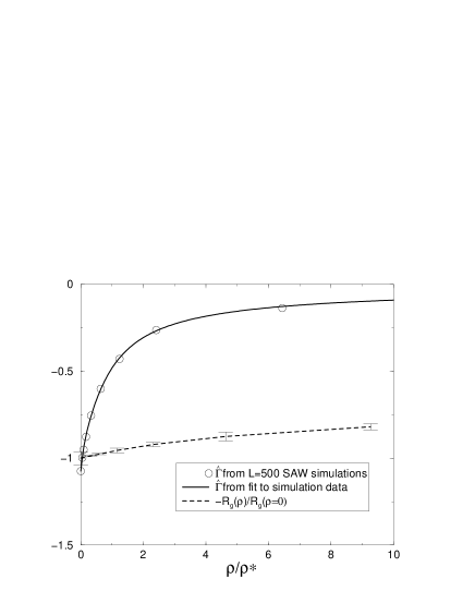
FIG. 2.: Relative adsorption $\hat{\Gamma}(\rho)$, in units of $R_{g}$, versus density. Circles denote direct computer simulations of $L=500$ SAW polymers near a single hard wall, and the line denotes the simple fit with the correct scaling behavior, given by Eq. (5). Also shown is the density dependence of the radius of gyration. In the semi-dilute regime $\hat{\Gamma}\approx-\xi\sim\rho^{0.770}$, while $R_{g}(\rho)/R_{g}(\rho=0)\sim\rho^{0.115}$

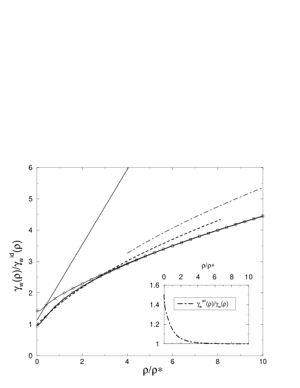
FIG. 3.: Polymer-wall surface tension $\gamma_{w}(\rho)$ divided by $\gamma_{w}^{id}(\rho)$. The full lines with square symbols are for interacting polymers and were calculated with Eq. (7), while the dotted line with circle symbols denotes the simpler expression of Eq. (8) which is only valid in the semi-dilute scaling regime, where $\gamma_{w}\sim\rho^{1.539}$. Also shown are two recent RG results[29]: the dashed line denotes the renormalized tree expansion, while the dot-dashed line denotes the asymptotic limit for an $\epsilon$-expansion. The solid line is from Eq. (9), a result derived from a recent PRISM calculation[31]. The inset shows the ratio of the full and simplified expressions for $\gamma_{w}(\rho)$. They coincide for higher densities but in the low density limit, the semi-dilute scaling expression overestimates the true surface tension by a factor $1.5$.

FIG. 4.: The effective AO radius $R_{AO}^{eff}$, given by Eq. (14), which would result in the same surface tension for an AO fluid around a sphere of radius $R_{c}$ as found for ideal polymers of size $R_{g}$. For infinite sphere size (i.e. a wall) $R_{AO}=(2/\sqrt{\pi})R_{g}$. As the relative sphere size $R_{c}/R_{g}$ decreases this effective parameter decreases due to the deformation of the polymers around a sphere. The symbols denote direct simulations $L=200$ ideal polymers on a lattice, taken from reference[12]. The small differences are due to the discrete nature of the lattice used in the simulations.

FIG. 5.: The polymer CM density profile $h(r)$ around a sphere for the ratios $q=R_{g}/R_{c}=0.67,1.05,1.68$ (graphs from top to bottom). For each sphere size the curves are for $\rho/\rho*=0.037,0.30,0.59,1.17,2.33$ (solid, dotted, dashed, long-dashed, and dot-dashed lines respectively). The depletion layer narrows with increasing density, just as was found for as single wall (compare with Fig. 1). The small vertical lines denote the position of the radius of the colloid. The polymers can wrap more easily around the smaller colloids, which explains why the CM profile penetrates further into the colloid for smaller $R_{c}/R_{g}$.

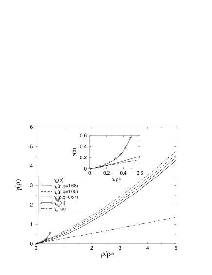
FIG. 6.: Surface tension for a planar wall, and for spheres with $q=0.67$, $q=1.05$ and $q=1.68$ as a function of density. We also include the planar surface tension of a HS fluid, with $R_{p}=R_{g}$ such that $\eta_{p}=\rho/\rho^{*}$. Inset: Blowup of the graph for low densities. The planar wall surface tension for interacting polymers, ideal polymers, and the HS system are compared.

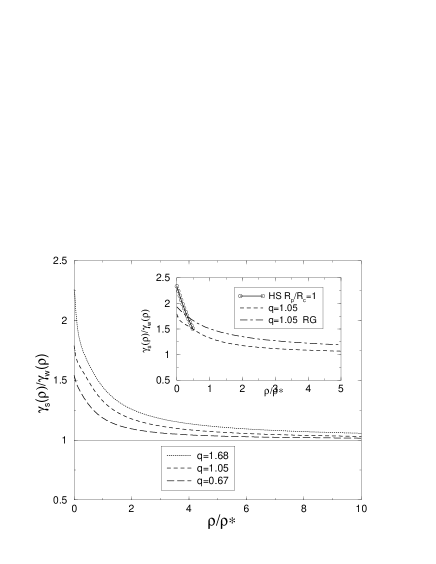
FIG. 7.: Ratio of surface tension of a sphere to the surface tension of a wall for spheres with $q=0.67$, $q=1.05$ and $q=1.68$. Inset: Comparison of an RG calculation[29] valid to lowest order in $q$, and our direct calculation for $q=1.05$. We also compare the ratio of the surface tension of a HS fluid around a single inserted sphere to the planar HS surface tension. The size-ratio is $1:1$, and $\eta_{p}=\rho/\rho^{*}$. The value at $\eta_{p}=0$ is equal to that of the AO model, given by Eq. (13).

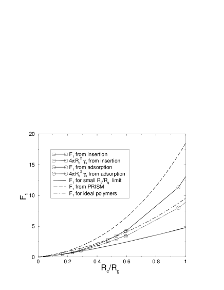
FIG. 8.: Insertion free energy $F_{1}$ for spheres of various radii $R_{c}$, in a polymer bath at $\rho/\rho^{*}=1.16$. For smaller $R_{c}/R_{g}$ a direct insertion method was used, while for larger $R_{c}/R_{g}$ the adsorption method was used. We also compare $4\pi R_{c}^{2}\gamma_{s}(\rho)$, the contribution to $F_{1}$ due to the creation of a depletion layer. For small $R_{c}/R_{g}$ this term is the dominant contribution to the insertion free energy $F_{1}$. Comparison is also made to an expression from RG theory, Eq. (22), valid in the small $R_{c}/R_{g}$ limit[28], with results from the PRISM approach[31] and with $F_{1}$ for ideal polymers, taken from Eq. (10). Note that for this density, the ideal and interacting results for $F_{1}$ cross each other at $R_{c}/R_{g}\approx 0.5$, below which it is easier to insert a spherical colloid into an interacting polymer solution than into a non-interacting one.

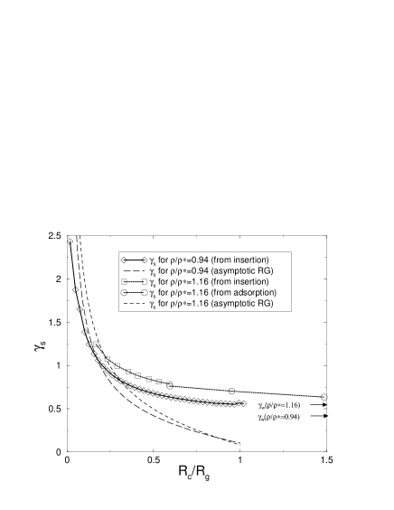
FIG. 9.: Surface tension $\gamma_{s}$ for spheres of different radius $R_{c}$, in a polymer bath at $\rho/\rho^{*}=1.16$, ($L=500$ SAW simulations) and for $\rho/\rho*=0.94$ ($L=2000$ SAW simulations). The insertion and the adsorption methods agree to within the expected statistical errors of our approach for $R_{c}=0.59R_{g}$. We also compare to an expression from RG theory, Eq. (22), valid in the small $R_{c}/R_{g}$ limit[28]. The arrows on the right depict the values of the planar surface tensions, valid as $R_{c}/R_{g}\rightarrow\infty$.

REFERENCES

- [1] S. Asakura and F. Oosawa, J. Chem. Phys. 22, 1255 (1954).
- [2] F.K.R. Li-In-On, B. Vincent, and F. A. Waite, ACS Symp. Ser. 9, 165 (1975).
- [3] F.L. Calderon, J. Bibette, and J. Bais, Europhys. Lett. 23, 653 (1993).
- [4] S.M. Ilett, A. Orrock, W.C.K. Poon, and P.N. Pusey, Phys. Rev. E, 51, 1344 (1995).
- [5] W.C.K. Poon et al., Phys. Rev. Lett. 83, 1239 (1999).
- [6] A. Weiss, K. D. Hörner, and M. Ballauff, J. Colloid Interface Sci. 213, 417 (1999).
- [7] A. Moussaid, W.C.K. Poon, P.N. Pusey, and M.F. Soliva, Phys. Rev. Lett. 82, 225 (1999).
- [8] E.H.A. de Hoog, H.N.W. Lekkerkerker, J. Schulz, and G.H. Findenegg, J. Phys. Chem. B 103, 10657 (1999).
- [9] Y.N. Ohshima et al. Phys. Rev. Lett. 78, 3963 (1997).
- [10] R. Verma, J.C. Crocker, T.C. Lubensky, and A.G. Yodh, Phys. Rev. Lett. 81, 4004 (1998).
- [11] C. Bechinger, D. Rudhardt, P. Leiderer, R. Roth and S. Dietrich, Phys. Rev. Lett. 83, 3960 (1999).
- [12] E.J. Meijer and D. Frenkel, Phys. Rev. Lett. 67, 1110 (1991); J. Chem. Phys. 100, 6873 (1994).
- [13] R. Tuinier, G. A. Vliegenthart, and H. N. W. Lekkerkerker, J. Chem. Phys. 113, 10768 (2000).
- [14] S. Asakura and F. Oosawa, J. Polym. Sci., Polym. Symp. 33, 183 (1958), A. Vrij, Pure Appl. Chem. 48, 471 (1976).
- [15] H.N.W. Lekkerkerker, W.C.K. Poon, P.N. Pusey, A. Stroobants and P.B. Warren, Europhys. Lett. 20, 559 (1992).
- [16] A. A. Louis, R. Finken, and J.P. Hansen, Europhys. Lett. 46, 741 (1999); M. Dijkstra, J. M. Brader and R. Evans, J. Phys.: Condens. Matter 11, 10079 (1999).
- [17] J.M. Brader and R. Evans, Europhys. Lett. 49, 678 (2000).
- [18] A.A. Louis, P.G. Bolhuis, J.P. Hansen and E.J. Meijer, Phys. Rev. Lett. 85, 2522 (2000).
- [19] P.G. Bolhuis, A.A. Louis, J.P. Hansen, and E.J. Meijer, J. Chem. Phys. 114, 4296 (2001).
- [20] P.G. Bolhuis, A.A. Louis, and J.P. Hansen, Phys. Rev. E. 64, 021801 (2001).
- [21] P.G. Bolhuis, A.A. Louis, to appear in Macromolecules (2001).
- [22] P.G de Gennes, Scaling Concepts in Polymer Physics, (Cornell University Press, Ithaca).
- [23] J. F. Joanny, L. Leibler, and P.G. de Gennes, J. Polym. Sci. Pol. Phys. 17, 1073 (1979).
- [24] R. Tuinier and H.N.W. Lekkerkerker, Eur. Phys. J. E 6, 129 (2001).
- [25] L. Shäfer Excluded Volume Effects in Polymer Solutions, (Springer Verlag, Berlin, 1999).
- [26] E. Eisenriegler, A. Hanke, and S. Dietrich, Phys. Rev. E 54, 1134 (1996).
- [27] A. Hanke, E. Eisenriegler and S. Dietrich, Phys. Rev. E. 59, 6853 (1999).
- [28] E. Eisenriegler, J. Chem. Phys. 113, 5091 (2000).
- [29] R. Maasen, E. Eisenriegler, and A. Bringer, J. Chem. Phys. 115, 5292 (2001).
- [30] M. Fuchs and K.S. Schweizer, Europhys. Lett. 51, 621 (2000).
- [31] M. Fuchs and K.S. Schweizer, Phys. Rev. E 64 021514 (2001).
- [32] M. Doi and S.F. Edwards, The Theory of Polymer Dynamics, (Oxford University Press, Oxford, 1986).
- [33] R.C. Tolman, J. Chem. Phys. 17, 118, 333 (1949).
- [34] J.S. Rowlinson and B. Widom, Molecular Theory of Capilarity, (Oxford University Press, Oxford 1989).
- [35] D. Frenkel and B. Smit, Understanding molecular simulations ( Academic Press, 1995).
- [36] . In our earlier work[18, 19, 20] we used instead of the correct value for the SAW polymers. This means a slight adjustment in the values of and in quoted in our papers. For example, the values quoted for should increase by a factor . We thank V. Krakoviack for pointing this out to us.
- [37] To compare with [27], who expressed their results in terms of , the end-to-end radius, we have used , the value expected for interacting polymers[32]. This is close to the ideal-polymer result .
- [38] Y. Mao, P. Bladon, H.N.W. Lekkerkerker and M.E. Cates, Mol. Phys. 92, 151 (1997)
- [39] See e.g. T. Ohta and Y. Oono, Phys. Lett. 89A, 460 (1982), or L. Shäfer, Macromolecules 15, 652 (1982). We use a modified expression from Y. Oono, Adv. Chem. Phys. 61, 301 (1985). The one remaining fit parameter is determined by fitting to the simulation data for SAW polymers, a procedure similar to that used when comparing to experiments[32], where the measured is used to set the fit parameter. In principle one can also extract from an RG calculation, so that the fit is not really necessary in the scaling limit[25]. However, we kept the fit form to make our results self-consistent for SAW polymers.
- [40] P.B. Warren, private communication.
- [41] P.G. de Gennes, C.R. Acad. Sci. Paris. B 288, 359 (1979).
- [42] R. Tuinier and H.N.W. Lekkerkerker, preprint (2001).
- [43] Y. Rosenfeld, Phys. Rev. Lett. 63, 980 (1989); J. Chem. Phys. 98, 8126 (1993).
- [44] R. Roth, R. Evans, and A.A. Louis, Phys. Rev. E. 64, 051202 (2001).
- [45] J. R. Henderson, Mol. Phys. 50, 741 (1983).
- [46] To correctly obtain the fully non-additive AO limit, the explicit in Eq. (18) should be equated with , while the packing fractions .
- [47] A.A. Louis, P. Bolhuis, and J.P. Hansen, Phys. Rev. E. 62, 7961 (2000); C.N. Likos, A. Lang, M. Watzlawek, and H. Löwen, ibid 63, 031206 (2001).
- [48] A.A. Louis, Phil. Trans. Roy. Soc. A 359, 939 (2001).
- [49] In the simulation we insert the colloid with its center a lattice site. We then check all the sites that are within the radius for overlap with one of the polymers. The number of these lattice sites, i.e. the volume occupied by the sphere can be transformed into an effective radius. This radius takes the discreteness effects partially into account, and is used in the analysis.
- [50] A.A. Louis, P.G. Bolhuis, E.J. Meijer, and J.P. Hansen, submitted (2001).