Aging Induced Multifractality

Abstract

We show that the dynamic approach to Lévy statistics is characterized by aging and multifractality, induced by an ultra-slow transition to anomalous scaling. We argue that these aspects make it a protoptype of complex systems.

The dynamic approach to Lévy statistics is still a poorly understood problem in spite of several attempts made at deriving it from intermittency[1, 2, 3] with several techniques ranging from Continuous Time Random Walk (CTRW)[4] to the Nakajima-Zwanzig projection method[5, 6]. This letter establishes that the dynamic approach implies aging, multiscaling and multifractality, thereby explaining, among other things, why this issue escaped so far a satisfactory understanding. The aim of this letter is to contribute to the comprehension of this delicate issue. Before addressing the problem from a more technical perspective that will be by necessity less accessible to a general audience, we want to illustrate the problem, and the solution of it afforded by this letter as well, with intuitive and qualitative arguments. To make our illustration as clear as possible, we adopt the same tutorial approach as that used by the authors working in the field of Cryptography[7], and we introduce two new archetypal individuals, Bob and Jerry. We hope that Bob and Jerry might have, with aging induced multifractality, the same fortune as Alice and Bob with Cryptography. These two individuals aim at realizing a process of diffusion of Lévy type, with an intensity that depends on secrete numbers known only to them. Since the width of the probability distribution does not depend only on time, but also on the intensity of the jumps made by the random walkers at any unit time, it is hard, in principle, to establish the time at which the diffusion process began, if the intensities of the jumps are not known. However, as we shall see, this is possible with Bob’s experiment, while it is impossible with Jerry’s experiment. In fact, Bob and Jerry realize Lévy diffusion in two different ways, and, as we shall see, Bob, who adopts the dynamic approach, allows us to predict the exact time at which he started the experiment, while it is not possible to guess the right starting time in the case of Jerry’s experiment. Bob generates a random sequence of pairs $\{\tau_{i},s_{i}\}$, with $i=0,1,...\infty$. The first number of each pair, $\tau_{i}$, is randomly drawn from the distribution

$$\psi(\tau)=\frac{(\mu-1)T^{\mu-1}}{(T+\tau)^{\mu}}.$$ (1)

The index $\mu$ has to fit the condition $\mu>2$, which ensures that the mean waiting time $\langle\tau\rangle$,

$$\langle\tau\rangle=\frac{T}{\mu-2},$$ (2)

is finite. Thus the number $T$ controls the intensity of $\langle\tau\rangle$. The second symbol, $s_{i}$, is a sign, $+$ or $-$, and it is obtained by tossing a fair coin. Let us imagine that this distribution is used to generate a diffusion process according to the following prescription. Bob, who has at his diposal a virtual infinite number of walkers, creates, for any of them, a sequence $\{\tau_{i},s_{i}\}$ and makes her travel with velocity $s_{i}W$ for the time $\tau_{i}$. Then Bob selects a number $r$ belonging to the interval $(0,\tau_{0}]$. The space travelled by the walker at time $t>\tau_{0}-r$ is given by

$$\begin{array}[]{ccc}x(t)&=&W[(\tau_{0}-r)s_{0}+\tau_{1}s_{1}+\cdots\\ &&+\tau_{N-1}s_{N-1}+(\tau_{N}-r^{\prime})s_{N}],\end{array}$$ (3)

where $r^{\prime}\equiv(\tau_{0}+\cdots+\tau_{N})-r-t$ and $N$ denotes the number of drawings made by Bob for his walker within the time interval $[0,t]$. At times $t<\tau_{0}-r$ ($N=0$) the space is given by

$$x(t)=W(\tau_{0}-r-r^{\prime})s_{0},$$ (4)

with $r^{\prime}=\tau_{0}-r-t$, yielding $x(0)=0$. Bob keeps secret both the value of $W$ and the value of $T$. He can try to make his diffusion process look older by increasing either both or only one of these secrete numbers. Furthermore, to erase any possible form of aging, he selects the number $r$ randomly. In fact, this has the effect of ensuring the stationary condition used by the authors of Refs[1, 4] to realize Lévy diffusion, under the form of Lévy walk[1], which seems to be more realistic than the flight prescription[2, 3].

To appreciate the properties of the Lévy walk, realized by Bob’s experiment, it is convenient to contrast it with Jerry’s experiment. Also Jerry has at his disposal a virtually infinite number of random walkers, whose position at $t=0$ is $x=0$, and he too, for any of his random walkers, selects an infinite sequence $\{x_{i}\}$. The numbers $x_{i}$ are drawn from a symmetric distribution, the positive numbers having the same probability as the negative numbers. For this reason Jerry does need the coin tossing to select $s_{i}$. Furthermore, Jerry makes his walker jump at any time step, by a jump of intensity $|x_{i}|$, in the positive or negative direction according to the sign of $x_{i}$. To be more precise, let us say that the distribution used by Jerry is $\Pi(x)$, defined through its Fourier transform,

$$\hat{\Pi}(k)=\exp(-b|k|^{\mu-1}),$$ (5)

and only Jerry knows the secrete value of $b$. The distribution of numbers used by Jerry is the well known Lévy distribution[8]: a stable distribution yielding a diffusion process, with the probability distribution $p_{L}(x,t)$, whose Fourier transform is

$$\hat{p}_{L}(k,t)=\exp(-b|k|^{\mu-1}t).$$ (6)

The time $t$ is the number of drawings, but it is so large as to be virtually indistiguishable from a continuous number. It is clear that the observation of Jerry’s diffusion process does not allow any observer to establish when he began his experiments. We assume that the observer, which might be a third archetypal individual, does not know the time at which Jerry began his diffusion. By means of the experimental observation he/she can only establish $bt$, and since $b$ is not known to him/her, he/she cannot determine the value of $t$. In other words, a broad distribution can be the consequence of Jerry starting his diffusion process at a very early time, but it can also be the consequence of a late beginning with much more intense jumps.

It is not so with Bob’s diffusion process. Let us see why. Let us consider, as in the case of Jerry’s experiment, a time $t$ very large. In the case of interest here, $\mu>2$, the mean waiting time, Eq. (2), is finite. Thus, the number of random drawings and coin tossings is very well approximated by $N=t/\langle\tau\rangle$. Using the Generalized Central Limit Theorem (GCLT) [9] we predict that Jerry’s experiment yields the same statistics as Bob’s experiment, Lévy statistics. However, this important theorem does not afford any clear indication about the time necessary to realize this statistics. The predictions of the GCLT theorems are realized[10] by the following expression for $p(x,t)$:

$$p(x,t)=K(t)p_{T}(x,t)\theta(Wt-|x|)+\frac{1}{2}\delta(|x|-Wt)I_{p}(t),$$ (7)

where $\theta$ denotes the Heaviside step function. We also note that

$$\lim_{t\rightarrow\infty}I_{p}(t)=\Phi_{\xi}(t)=\left(\frac{T}{T+t}\right)^{\mu-2},$$ (8)

$p_{T}(x,t)$ is a distribution that for $t\rightarrow\infty$ becomes identical to the anti-Fourier transform of Eq. (6), and $K(t)$ is a time-dependent factor ensuring the normalization of the distribution $p(x,t)$.

We observe that at any time $t$, no matter how arbitrarily large, it is possible to find a significant number of Bolb’s walkers, with $\tau_{0}-r>t$, namely, walkers for which Bob has not yet drawn the second pair of stochastic numbers. This probability is expressed by[11]

$$\Phi_{\xi}(t)=\frac{1}{\langle t\rangle}\int_{t}^{\infty}(t^{\prime}-t)\psi(t^{\prime})dt^{\prime}.$$ (9)

It is interesting to notice that, due to the fact that Bob decides the motion direction by tossing a coin, the function $\Phi_{\xi}(t)$ is the correlation function of the variable $\xi(t)$, namely, the fluctuating velocity created by Bob’s experiment. The number of walkers contributing to the propagation front is slightly larger. However, it is straightforward to prove with arguments similar to those used by Zumofen and Klafter[4] that in the asymptotic time limit $I_{p}(t)$ becomes identical to $\Phi_{\xi}(t)$, thereby accounting for the former of the two equalities of Eq. (8). The latter is easily accounted for by plugging $\psi(\tau)$ of Eq. (1) into Eq. (9).

On the basis of these arguments we reach the conclusion that in the asymptotic time limit Eq. (7) becomes identical to (see [5] for earlier derivation)

$$p(x,t)=p_{L}(x,t)\theta(Wt-|x|)+\frac{1}{2}\delta(|x|-Wt)\Phi_{\xi}(t).$$ (10)

This equation, although valid only in the asymptotic time limit, is very convenient for the theoretical arguments of this letter. First of all, it allows us to determine the age of the diffusion experiment created by Bob, even if Bob adopts the stationary condition[1, 4] and keeps secret the values of $W$ and $T$. To do so, we measure the distance of one ballistic peak from the other, the diffusion coefficient $b$ of $p_{L}(x,t)$ of Eq. (6) and the intensity of the two ballistic peaks. All these three quantities can be expressed in terms of the unknown quantities, $t$, $W$ and $T$. The distance between the two peaks is: $2Wt$; the diffusion coefficient is given by: $b=W(TW)^{\mu-2}sin[(\pi(\mu-2)/2]\Gamma(3-\mu))$ [12] and the peak intensity by Eq. (8). The age of Bob’s experiment can be revealed by means of experimental observation, thanks to the breakdown of homogeneity (multi-scaling), caused by the ultra-slow relaxation of $\Phi_{\xi}(t)$. At the intuitive level of this first part of the letter, we can say that aging causes inhomogeneity.

Let us now move to a more technical level of description. We share the vision of Khinchin[13] about the close connection between ordinary statistical mechanics and the ordinary Central Limit Theorem. There is, on the other hand, a close connection between statistical equilibrium and scaling of a diffusion process. The latter property is expressed by

$$p(x,t)=\frac{1}{t^{\delta}}F(\frac{x}{t^{\delta}}).$$ (11)

In fact, this property means that the probability density at different times can be expressed in terms of the same time independent property $F(y)$. The case of ordinary statistical mechanics corresponds to $\delta=1/2$ with $F(y)$ being a Gaussian function of $y$. The case under study in this paper is not ordinary because $F(y)$ is a Lévy distribution and the scaling parameter $\delta$ is given by

$$\delta=\frac{1}{\mu-1}.$$ (12)

This thermodynamic condition, however, is the asymptotic limit of a very slow transition, driven by the correlation function $\Phi_{\xi}(t)$ of Eq. (8), whose lifetime, in the case here under study, with $2<\mu<3$, is infinite. For a further discussion of this extremely slow transition from dynamics to thermodynamics, the reader can consult also Ref. [14]. Although this process of transition to thermodynamics, or aging, is extremely slow, with virtually an infinite lifetime, it is not easy to detect by mean of the current techniques of analysis of time series, which rest on the observation of a single sequence (see for instance Ref. [15]). Here we show that it turns out to be difficult even with the most advanced method of scaling detection, the method of Diffusion Entropy (DE) [15]. The first step of all these techniques, including the DE method, is based on deriving the random walkers required by Bob’s experiments from a single sequence. We use Bob’s algorithm to create a single, virtually infinite, trajectory. Then we span infinitely many portions of this sequence moving along the sequence a window of width $t$. The selected walking trajectories are shifted in such a way as to make them start at $x=0$ at $t=0$. These trajectories tends to depart the ones from the others, as an effect of their partially random character, and this spreading is described by $p(x,t)$, evaluated numerically with a proper partition of the $x$-axis. At this stage, rather than evaluating the variance, which leads to a wrong scaling in the Non-Gaussian case[16], we evaluate the Shannon entropy

$$S(t)=-\int_{-\infty}^{+\infty}p(x,t)\log(p(x,t)).$$ (13)

In the case when the scaling condition of Eq. (11) applies, by plugging Eq. (11) into Eq. (13) we get

$$S(t)=A+\delta\log(t),$$ (14)

with $A$ being a constant whose explicit expression is of no interest here. Fig. 1 proves that the DE method is successful in detecting the predominant asymptotic scaling of Eq. (12). This is a flattering result, since the methods based on the variance measurement cannot reveal this Lévy scaling. However, it is not easy to relate Fig. 1 to the slow transition process described by Eq. (10) [10].

We can go beyond the limitations of the DE method of analysis detecting the multifractal properties generated by the aging process itself. To reveal the emergence of these multifractal properties we rest on Eq. (10) and on a procedure reminiscent of that of Nakao[17]. This author proved in fact that a truncated Lévy process yield bifractal properties. It has to be pointed out, however, that there is a deep difference between the case considered by Nakao and the dynamic truncation of this letter. The effect observed by Nakao has to do with the ultraslow convergence to Gaussian statistics discussed some years ago by Mantegna and Stanley[18], observed independently by the authors of Ref.[19]. The effect here discussed is instead an ultraslow convergence to Lévy statistics. Moreover, as we have seen, our transition process has an infinite lifetime, while the lifetime of that of Refs.[18, 19], although impressively large, is finite.

To study the multifractal properties associated to the dynamic approach to Lévy processes, we follow the prescriptions of Refs.[20, 21]. We study theoretically and numerically the fractional moment $\langle|x|^{q}\rangle$, which is expected to yield

$$\langle|x|^{q}\rangle=\int_{\infty}^{+\infty}p(x,t)|x|^{q}dx\approx t^{\xi_{q}}.$$ (15)

The power index $\xi_{q}$ plays a critical role. According to the theory of Refs. [20, 21], $\xi_{q}$ as a function of $q$, would be a straight line if the monofractal condition applied, while its deviation from a straight line signals the occurrence of multifractal properties. Using the theoretical prediction of Eq. (10) it is straigforward to predict that

$$\xi_{q}=\delta q,$$ (16)

for $q<\mu-1$, and

$$\xi_{q}=q-\mu+2,$$ (17)

for $q>\mu-1$. These theoretical predictions are very satisfactorily supported by the numerical results, as proved by Fig. 2.

In conclusion, we define aging the process of transition from dynamics to thermodynamics when this transition has an infinite lifetime[22, 23]. If it had a finite lifetime, it would be possible to make an observation at times so large as to make the scaling condition of Eq. (11) virtually exact. This condition, in turn, plugged into Eq. (15), would make Eq. (16) valid for all $q$’s, and not not only for the small ones. This means that no aging is equivalent to the condition of monofractal statistics. If, on the contrary, aging exists, the diffusion process becomes bifractal. This is what we mean by aging induced multifractality. We propose aging as a paradigm for the living state of matter. This has to do with the widely accepted conviction (see, for instance, Ref.[24]) that life is a balance of order and randomness. This paper shows that aging, as we do mean it, is an attractive expression of this balance.

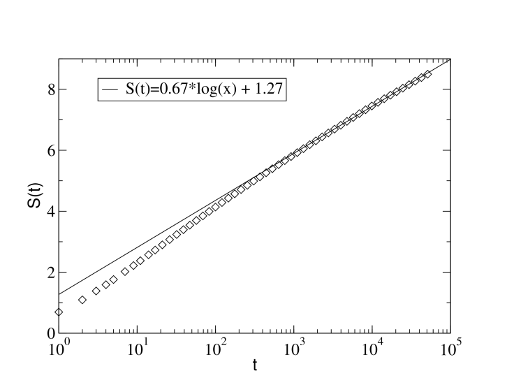
FIG. 1.: Diffusion Entropy as a function of time t. Dots: numerical evaluation of $S(t)$ for Bob’s experiment with $\mu=2.5$, $T\approx 1.0$. Bob’s walkers are derived from a single trajectory of total lenght 25,918,673 time units (see the text for details). The solid line represents a best fit, in the asymptotic regime, of the theoretical prediction $S(t)=2/3\log(t)+const$.

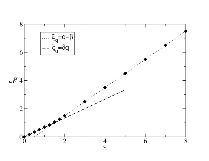
FIG. 2.: Multifractal index $\xi_{q}$ as a function of q. Dots: numerical evaluation of $\xi_{q}$ for Bob’s experiment (dynamical truncated Lévy process) using the same data as those of Fig.1. Dashed line: $\xi_{q}=\delta q$, with $\delta=2/3$ according to (12); dotted line: $\xi_{q}=q-\beta$, with $\beta\equiv\mu-2=0.5$.

REFERENCES

- [1] T. Geisel, J. Nierwetberg, and A. Zacherl, Phys. Rev. Lett. 54, 616 (1985).
- [2] M.F. Shlesinger, J. Klafter, Phys. Rev. Lett. 54, 2551 (1985).
- [3] M.F. Shlesinger, B.J. West, J. Klafter, Phys. Rev. Lett. 58, 1100 (1987).
- [4] G. Zumofen and J. Klafter, Phys. Rev. E 47, 851 (1993).
- [5] P. Allegrini, P. Grigolini, B.J. West, Phys. Rev. E 54, 4760 (1996).
- [6] M. Bologna, P. Grigolini, and J. Riccardi, Phys. Rev. E 60, 6435 (1999).
- [7] B. Schneider, Applied Cryptograpy, 2nd ed, John Wiley, New York (1996)
- [8] E. W. Montroll and M. F. Shlesinger, in Nonequilibrium Phenomena II, From Stochastics to Hydrodynamics, eds. J.L. Lebowitz and E.W. Montroll, Elsevier Science Publishers, New York (1984).
- [9] B. V. Gnedenko and A. N. Kolmogorov, Limit Distributions for Sums of Independent Random Variables, Addison Wesley, (1954).
- [10] G. Bramanti, P. Grigolini, M. Ignaccolo, G. Raffaelli, work in progress.
- [11] T. Geisel, in Lévy Flights and Related Topics in Physics, Proceedings, Nice, France 1994, Lecture Notes in Physics 450, Springer, Berlin, p. 153.
- [12] M. Annunziato, P. Grigolini, Phys. Lett. A 269, 31 (2000).
- [13] A.I. Khinchin, Mathematical Foundations of Statistical Mechanics Dover Publications, Inc. New York (1949).
- [14] M. Ignaccolo, P. Grigolini, A. Rosa, Phys. Rev. E 64, 026210 (2001).
- [15] N. Scafetta, P. Hamilton, P. Grigolini, Fractals, 9 193 (2001).
- [16] N. Scafetta, V. Latora and P. Grigolini, work in progress.
- [17] H. Nakao, Phys. Lett. A 266, 282 (2000).
- [18] R.N. Mantegna and H.E. Stanley, Phys. Rev. Lett., 73, 2946 (1994).
- [19] E. Floriani, R. Mannella, P. Grigolini, Phys. Rev E 52, 5910 (1995).
- [20] R. Benzi, G. Paladin, G. Parisi, A, Vulpiani, J. Phys. A 17, 3521 (1984).
- [21] G. Paladin, A. Vulpiani, Phys. Rep. 156, 149 (1987).
- [22] Spin Glasses and Random Fields, edited by A.P. Young, Series on Directions in Condensed Matter Physics, 12, World Scientific, Singapore (1998).
- [23] We do not claim that our definition of aging corresponds to the spin-glass property with the same name (see Ref. [22] for a sample of papers on this literature). We do not rule out, however, the possibility of an interesting connection.
- [24] R.V. Sole, B. Goodwin, Signs of Life: How Complexity Pervades Biology, Basic Books, New York (2001).