Dynamics and Configurational Entropy in the LW Model for Supercooled Orthoterphenyl

Abstract

We study thermodynamic and dynamic properties of a rigid model of the fragile glass forming liquid orthoterphenyl. This model, introduced by Lewis and Wahnström in 1993, collapses each phenyl ring to a single interaction site; the intermolecular site-site interactions are described by the LJ potential whose parameters have been selected to reproduce some bulk properties of the orthoterphenyl molecule. A system of $N=343$ molecules is considered in a wide range of densities and temperatures, reaching simulation times up to 1 $\mu s$. Such long trajectories allow us to equilibrate the system at temperatures below the mode coupling temperature $T_{c}$ at which the diffusion constant reaches values of order $10^{-10}\>cm^{2}/s$ and thereby to sample in a significant way the potential energy landscape in the entire temperature range. Working within the inherent structures thermodynamic formalism, we present results for the temperature and density dependence of the number, depth and shape of the basins of the potential energy surface. We evaluate the total entropy of the system by thermodynamic integration from the ideal –non interacting– gas state and the vibrational entropy approximating the basin free energy with the free energy of $6N-3$ harmonic oscillators. We evaluate the configurational part of the entropy as a difference between these two contributions. We study the connection between thermodynamical and dynamical properties of the system. We confirm that the temperature dependence of the configurational entropy and of the diffusion constant, as well as the inverse of the characteristic structural relaxation time, are strongly connected in supercooled states; we demonstrate that this connection is well represented by the Adam-Gibbs relation, stating a linear relation between $\log D$ and the quantity $1/TS_{c}$. This relation is found to hold both above and below the critical temperature $T_{c}$ —as previously found in the case of silica— supporting the hypothesis that a connection exists between the number of basins and the connectivity properties of the potential energy surface.

I INTRODUCTION

Understanding the dynamic and thermodynamic properties of supercooled liquids is one of the more challenging tasks of condensed matter physics (for recent reviews see Refs. [1, 2, 3, 4] and references therein). A significant amount of experimental [5, 6, 7, 8, 9], numerical [10] and theoretical work [11, 12, 13, 14, 15] is being currently devoted to the understanding of the physics of the glass transition and to the associated slowing down of the dynamics. Among the theoretical approaches, an important role has been played by the mode coupling theory (MCT) [11, 12], which, interpreting the glass transition as a purely dynamical phenomenon, has constituted a significant tool for the interpretation of both experimental[5, 9, 16, 17, 18, 19] and numerical simulation results[20, 21, 22] in weakly supercooled states.

In the last years the study of the topological structure of the potential energy (hyper-) surface (PES)  [23] and the connection between the properties of the PES and the dynamical behavior of glass forming liquids has become an active field of research. Building on the inherent structure (IS) thermodynamic formalism proposed long time ago by Stillinger and Weber [23], the PES can be uniquely partitioned in local basins and properties of the basins explored in supercooled states (average basin depth and basin volume), have been quantified. Studies have mainly focused on two fundamental questions: (i) which are the basins relevant for the thermodynamics of the system, i.e., which are the basins populated with largest probability? and (ii) which are the topological properties of the regions of the PES actually explored by the system during its dynamics? From this point of view, the PES approach has somehow unified, at least on a phenomenological level, the thermodynamic and dynamic approaches to the glass transition.

Numerical analysis of the PES has shown that trajectories in configuration space can be separated into intra-basin and inter-basin components [24, 25]. The time scales of the two components become increasingly separated on cooling. The intra-basin motion has been associated with the high-frequency vibrational dynamics, while the structural relaxation ($\alpha$-relaxation) has been related to the process of exploration of different basins. It has also been shown that on lowering $T$, the system populates basins of lower and lower energy[26]. The $T$ dependence of the depth of the typical sampled basins follows a $1/T$ law [27, 28, 29] for fragile liquids, and, for strong liquids, it appears to approach a constant value on cooling [30]. The number of basins $\Omega$ as a function of the basin depth $e_{IS}$ has also been recently evaluated for a few models [31, 32, 28, 30, 33, 27], opening the possibility of calculating the so-called configurational entropy $S_{c}$ and its $T$ dependence. $S_{c}$, defined as the logarithm of the number of accessible basins $S_{c}\equiv k_{B}\log\Omega$, has been successfully compared with theoretical predictions[13, 34]. At the same time, the approaches and the techniques developed for the analysis of the PES of structural glasses have spread to the field of disordered spin systems, where similar calculations have been performed[35] and similar conclusions have been reached. The evaluation of $S_{c}$ for models of glass-forming liquids allows to numerically check, in a very consistent way, the relation between $S_{c}$ and the systems characteristic time $\tau$, proposed by Adam and Gibbs [36], and recently “derived” in a novel way[14]. Numerical support for a relation between the $T$ dependence of $S_{c}$ and the $T$ dependence of $\tau$, although limited to very few models, is providing new physical insight on the connection between thermodynamics and long time dynamical properties. The ideas developed within the inherent structure formalism have also been generalized to out-of-equilibrium conditions where the slow aging dynamics has been interpreted as the process of searching for basins of increasingly deep energy  [37, 38, 39, 40].

In this paper we study the properties of the PES for a rigid model (LW) of the fragile glass former orthoterphenyl, first introduced by Lewis and Wahnström [41] and recently revisited by Rinaldi et al.[42]. We have studied the properties of the PES in a temperature range in which the diffusion coefficient varies by more than four orders of magnitudes for five different density values. This work attempts to build a bridge between models of more direct theoretical interest, like Lennard Jones (LJ) and soft spheres, and models which appear to reproduce, even if in a crude way, properties of complex materials. In this respect, orthoterphenyl is the best candidate, being one of the most studied glass forming liquids [17]. The LW model is a three-sites model, with intermolecular site-site interactions described by the LJ potential. This model is among the simplest models for a nonlinear molecule. The limitation constituted by the fact that it does not take into account the internal molecular degrees of freedom (see [43] for a more realistic model), is overruled by the observation that its simplicity —it can be considered as an atomic LJ with constraints— allows one to reach simulation times of the order of $\mu s$. Hence a significant sampling of the PES in a large temperature and density range is possible. Moreover, this model constitutes an ideal bridge between simple atomic models and molecular models, being possible to treat it under several approximations[42].

The paper is structured as follows: In Sec. II we briefly recall the main results of the IS formalism. In Sec. III we show the calculation of the configurational entropy as a difference between the total entropy and the vibrational entropy. In Sec. IV we give some numerical details. We present our results in Sec. V, which is divided into subsections detailing the calculation of the total entropy by thermodynamical integration from the ideal gas state, the study of the vibrational properties of the PES and the calculation of the configurational entropy. In the end we study the link between configurational entropy and the diffusion constant, investigating the validity of the Adam-Gibbs equation. In Sec. VI we finally discuss our results and we draw some conclusions. In Appendix A we report the analytical calculation of the total entropy of a system of LW molecules in the non-interacting “ideal gas” limit.

II Inherent Structure Thermodynamics formalism

In this section we briefly review the IS formalism in the NVT ensemble [23, 44], the extension to the NPT ensemble poses no particular problems [23]. This formalism has become an important tool in the numerical analysis of classical models since it is numerically possible to calculate in a very precise way the inherent structures (defined as the local minima of the PES) and hence compare the theoretical predictions with the numerical results. Given an instantaneous configuration of the system, a steepest descent path along the potential energy hypersurface defines the closest IS.

In the IS formalism, the partition function of a system is written as a sum over all the PES basins. Basins of given IS energy contribute non-negligibly to the total sum if their IS energy is very low, if their volume is very large and/or if they are highly degenerate, i.e. several basins are characterized by this IS energy. This corresponds to partition the phase space in the local energy minima of the PES and their basins of attraction. Such a partition is motivated by the fact that in supercooled states, the typical time scales of the intra basin and inter basin dynamics differ by several orders of magnitude and hence the separation of intrabasin and interbasin variables becomes meaningful.

In the $6N$-dimensional configuration space, the partition function $Z$ for a system of $N$ rigid molecules can be written as:

$$Z=\frac{\Lambda_{x}\Lambda_{y}\Lambda_{z}}{\lambda^{3N}}\int d{\bf q}^{N}\exp(-V({\bf q}^{N})/k_{B}T),$$ (1)

where ${\bf q}^{N}$ denotes the positions and orientations of the molecules, $V({\bf q}^{N})$ is the potential energy , $I_{\mu}$, with $\mu=x,y,z$, are the principal moments of inertia of the molecule, ${\Lambda}_{\mu}\equiv(2\pi I_{\mu}k_{B}T)^{1/2}/h$, and $\lambda\equiv h(2\pi mk_{B}T)^{-1/2}$ is the de Broglie wavelength.

Let $\Omega(E_{IS})$ denote the number of minima with energy $E_{IS}$, and $f(T,E_{IS})$ the average free energy of a basin with basin depth $E_{IS}$. $f(T,E_{IS})$, which takes into account both the kinetic energy of the system and the local structure of the basin with energy $E_{IS}$, is defined by:

$$f(T,E_{IS}) \equiv -k_{B}T\ln\left[\frac{\Lambda_{x}\Lambda_{y}\Lambda_{z}}{\lambda^{3N}}\frac{1}{\Omega(E_{IS})}\right.\times$$ (3)

$$\left.\sum_{\mbox{basins}}\int_{R_{\mbox{basin}}}d{\bf q}^{N}\exp(-(V-E_{IS})/k_{B}T)\right],$$

where $R_{basin}$ is the configuration volume associated with the specific basin. The partition function can then be rewritten as a sum over all basins in configurational space, i.e.

$$Z=\sum_{E_{IS}}\Omega(E_{IS})\exp\left({-\frac{E_{IS}+f(T,E_{IS})}{k_{B}T}}\right)$$ (4)

$$=\sum_{E_{IS}}\exp\left({-\frac{-TS_{c}(E_{IS})+E_{IS}+f(T,E_{IS})}{k_{B}T}}\right)$$ (5)

where the configurational entropy $S_{c}(E_{IS})$ has been defined as

$$S_{c}(E_{IS})\equiv k_{B}\ln\left[\Omega(E_{IS})\right].$$ (6)

In the thermodynamic limit, the free energy of the liquid can be calculated using

$$F\left[e_{IS}(T)\right]=e_{IS}(T)+f\left[T,e_{IS}(T)\right]-TS_{c}\left[e_{IS}(T)\right],$$ (7)

where $e_{IS}(T)$, the average value of the IS energy at temperature $T$, is the solution of the saddle point equation

$$1+\frac{\partial f}{\partial E_{IS}}-T\frac{\partial S_{c}}{\partial E_{IS}}=0.$$ (8)

The liquid free energy expression Eq. (7) has a clear interpretation. The first term in Eq. (7) takes into account the average energy of the PES minimum visited, the second term describes the volume of the corresponding basin of attraction and the kinetic energy, and the third term is a measure of the multiplicity of the basin.

It can be rigorously shown [29, 44, 27] that, if the density of state $\Omega(E_{IS})$ is Gaussian, and if the basins have approximately the same shape or are, to a good degree, harmonic, the important relation holds

$$e_{IS}(T)\propto\frac{1}{T}.$$ (9)

On lowering $T$, basins with lower $E_{IS}$ energies and lower degeneracy are populated, i.e., both $e_{IS}$ and $S_{c}$ decrease with $T$.

III Evaluation of the configurational entropy

The Eq. (7) provides a natural starting point for a numerical evaluation of the configurational entropy. Indeed, the free energy $F(T,V)$ per molecule can be split in the usual way as a sum of an energy and an entropic contribution. Considering Eq. (7) we write:

$$F(T) = E(T)-TS(T)$$ (10)

$$= -TS_{c}(T)+e_{IS}(T)+E_{v}(T)-TS_{v}(T)$$ (11)

where the index $v$ indicates the vibrational quantities (intra-basin components). In order to evaluate these quantities we calculate the basin free energy as the free energy of $6N-3$ independent harmonic oscillators [32] plus a contribution that takes into account the basin anharmonicities. Then we can write

$$E(T) = \left(6-\frac{3}{N}\right)\frac{k_{B}T}{2}+e_{IS}(T)+U_{\rm anh}(T),$$ (12)

$$S(T) = S_{v}(T)+S_{c}(T)$$ (13)

$$= S_{\rm harm}(T)+S_{\rm anh}(T)+S_{c}(T),$$ (14)

and

$$S_{\rm harm}=\left(6-\frac{3}{N}\right)-\frac{1}{N}\sum_{n=1}^{6N-3}\ln\left[\frac{\hbar\;\omega_{n}(T)}{k_{B}T}\right],$$ (15)

where the frequencies $\omega_{n}$ are the square root of the eigenvalues of the Hessian matrix calculated in the inherent structures.

Thus, the total entropy is the sum of two contributions: $S_{c}(T)$ which accounts for the multiplicity of basins of depth $e_{IS}(T)$, and $S_{v}(T)$ which accounts for the “volume” of the basins. The last equations give us, in a very transparent way, the physical meaning of the partition of the PES; moreover, they provide us a very efficient way to calculate the configurational entropy as a difference between the total energy of the system and the vibrational entropy.

The total entropy $S$ can be evaluated via thermodynamic integration, starting from a known reference point. Every variation of total entropy can be generally written as the sum of variation along isochores and isotherms in the form:

$$\Delta S=\Delta S_{V}+\Delta S_{T}.$$ (16)

Then the change of entropy along an isochore between two temperatures $\bar{T}$ and $T$ is

$$\Delta S_{V} = S(V,T)-S(V,\bar{T})$$ (17)

$$= \int_{\bar{T}}^{T}\frac{dT^{\prime}}{T^{\prime}}\;c_{v}(T^{\prime})$$ (18)

and the change along an isotherm between two volumes $\bar{V}$ and $V$ is

$$\Delta S_{T} = S(V,T)-S(\bar{V},T)$$ (19)

$$= \frac{1}{T}\left[E(V,T)-E(\bar{V},T)+\int_{\bar{V}}^{V}d\bar{V}P(\bar{V},T)\right].$$ (20)

In the present case, to evaluate the total entropy of the liquid we start from the known expression of the ideal gas of LW molecules, reviewed in Appendix A. To evaluate the basin free energy $f\left[T,e_{IS}(T)\right]$, we select as reference point the free energy of $(6N-3)$ independent harmonic oscillators (whose distribution of frequencies can be calculated evaluating the eigenvalues of the Hessian matrix evaluated in the IS structure) and add corrections to take into account the basin anharmonicities.The harmonic contribution to the entropy is given by Eq. (15).

Assuming that the anharmonic contribution is independent from the basin depth, the anharmonic corrections to the entropy at $T$ can be calculated integrating the quantity $dU_{\rm anh}/T$, where $U_{\rm anh}$ is implicitly defined in Eq. (12), from $T=0$ to $T$ (see Eq. (17)).

IV NUMERICAL DETAILS

The LW model is defined by the spherical potential

$$V(r)=4\epsilon\,\left[\left({{\sigma}\over{r}}\right)^{12}-\left({{\sigma}\over{r}}\right)^{6}\right]+\lambda_{1}+\lambda_{2}\,r,$$ (21)

with $\epsilon=5.276$ $kJ/mol$, $\sigma=0.483$ nm $\lambda_{1}=0.461$ $kJ/mol$ and $\lambda_{2}=-0.313$ $kJ/(mol~{}nm)$. The parameters of the potential are selected to reproduce some bulk properties of the OTP molecule [41] such as the temperature dependence of the diffusion coefficient and the structure. The values of $\lambda_{1}$ and $\lambda_{2}$ are selected in such a way the potential and its first derivative are zero at $r_{c}=1.2616$ $nm$. Such a potential is characterized by a minimum at $r=0.542$ $nm$ of depth $-4.985$ $kJ/mol$. The integration time step is $0.01$ ps. The shake algorithm is implemented to account for the molecular constraints.

We study a (N,V,E) system composed by $N=343$ molecules ($1029$ LJ interaction sites) at 5 different densities (see Table I) for several temperatures at each density (Table II). The total simulation time is quite long, exceeding 10 $\mu s$. We take care to check the thermalization of the system at the lowest temperatures; the production run follows a thermalization run whose length is comparable to the relaxation time at the considered thermodynamical point. We are able to thermalize the system at temperatures at which the diffusion constant reaches values very low, of order 10^-10 cm²/s, 10⁴ smaller then at ambient temperature.

Two additional simulations are performed to connect the range of densities and temperature studied with the ideal gas reference point. The system at density $\rho_{4}$ is simulated for temperatures ranging from 250 to 5000 K to evaluate the $T$ dependence of the potential energy. A second set of simulations at constant $T$ ($T=5000$ K) in the volume range $10^{2}-10^{5}$ nm³ is performed to calculate the excess pressure ( i.e. the pressure beyond the ideal gas contribution).

To calculate the inherent structures visited in equilibrium we perform conjugate gradient minimizations to locate the closest local minima on the PES. We use a tolerance of $10^{-15}$ kJ/mol in the total energy for the minimization. For each thermodynamical point we minimize at least $100$ configurations and we diagonalize the Hessian matrix of at least $50$ configurations to calculate the density of states. The Hessian is calculated choosing for each molecule the center of mass and the angles associated with rotations around the three principal inertia axis as coordinates.

V RESULTS

A Dependence of the total entropy on $T$ and $\rho$

To estimate the total entropy for the model we proceed in three steps as shown in Fig. 1. The thermodynamic path has been chosen to avoid the liquid-gas first order line.

(1) Integration along the isotherm $T_{0}$ = 5000 K from ($T_{0}$,$V=\infty$) (perfect gas) to ($T_{0}$, V₄=118.35 nm³), corresponding to point $C_{0}$ in Fig. 1. The ideal gas contribution to the total entropy is discussed in Appendix A. The entropy at $C_{0}$ can be calculated as

$$S(T_{0},V_{4})-S_{id}(T_{0},V_{4})=$$ (22)

$$\frac{U(T_{0},V_{4})}{T_{0}}+\int_{\infty}^{V_{4}}\frac{dV}{T_{0}}P_{ex}(V,T_{0}),$$ (23)

where $P_{ex}$ is the pressure that exceeds the pressure of the ideal gas, i.e. the contribution to the pressure due to the interaction potential and $U$ is the system potential energy. The values of the pressure $P_{ex}(T=T_{0},V,N=343)$ as a function of $V$ are reported in Fig.2 (a). $P_{ex}(T=T_{0},V,N=343)$ has been fit using the virial expansion

$$P_{ex}(T=T_{0},V,N=343)=\sum_{k=1}^{4}a_{k}V^{-(k+1)}.$$ (24)

The $a_{k}$ values are reported in Table III, from which we estimate the first virial coefficient at $T_{0}$

$$B_{2}(T_{0})=a_{1}/(k_{B}T_{0}N^{2})=0.596\;{\rm nm^{3}}.$$ (25)

In Fig.2 (b) we plot the potential energy as a function of volume along the $T=T_{0}$ isotherm.

The total entropy at the reference point $C_{0}$ is $S(C_{0})=$ 294.8 J/( mol K ), resulting from the sum of three contributions

$$S_{id}(C_{0})=339.03\;J/(molK),$$ (26)

$$\int_{\infty}^{V_{4}}\frac{dV}{T_{0}}P_{ex}(V,T_{0})=-44.9\;J/(molK),$$ (27)

and

$$\frac{U(C_{0})}{T_{0}}=0.64\;J/(molK)$$ (28)

(2) Integration along the isochore $V=V_{4}$ from $T_{0}$ to $T^{*}=380$ K, corresponding to the point $C_{1}$ in Fig.1. To evaluate the entropy along this isochore we use

$$S(T^{*},V_{4}) = S(T_{0},V_{4})+3R\;\log(T^{*}/T_{0})$$ (29)

$$+ \int_{T_{0}}^{T^{*}}\frac{dT}{T}\frac{\partial U(V_{4},T)}{\partial T}.$$ (30)

Fig. 3 (a) shows the potential energy for the $V=V_{4}$ isochore. To calculate the integral in Eq. (30), we fit the potential energy using the functional form which best interpolates the calculated points

$$U(V_{4},T)=u_{0}+u_{1}T^{3/5}+u_{2}T,$$ (31)

obtaining the values $u_{0}=-94.405,u_{1}=0.533,u_{2}=0.00183$ (energy in $kJ/mol$).

The total entropy at the reference point $C_{1}$ is $S(C_{1})=$ 191.8 J/( mol K ), resulting from the sum of three contributions:

$$S(C_{0})=308.6\;J/(molK),$$ (32)

$$3R\;\log(T/5000)=-64.3\;J/(molK),$$ (33)

and

$$\int_{T_{0}}^{T^{*}}\frac{dT}{T}\frac{\partial U(V_{4},T)}{\partial T}=-52.5\;J/(molK).$$ (34)

(3) Integration along the isotherm $T^{*}$ from $V_{4}$ to a “generic” $V$. To determine the total entropy difference for all studied densities we calculate

$$S(T^{*},V)-S(T^{*},V_{4}) = S_{id}(T^{*},V)-S_{id}(T^{*},V_{4})$$ (35)

$$+ \frac{1}{T^{*}}\left[U(T^{*},V)-U(T^{*},V_{4})\right]$$ (36)

$$+ \int_{V_{4}}^{V}\frac{dV^{\prime}}{T^{*}}P_{ex}(T^{*},V^{\prime}).$$ (37)

Figs. 3 (b) and (c) show respectively the potential energy and the excess pressure as a function of volume at $T=T^{*}$. For convenience we fit $P_{ex}$ with a third order polynomial

$$P_{ex}(T^{*},V)=\sum_{k=1}^{4}p^{*}_{k}V^{k-1},$$ (38)

where the values of the coefficients $p^{*}_{k}$ are given in Table III. The resulting total entropy at $T^{*}$ for all studied densities is reported in Table IV. These values are used as reference entropies for the $T$ dependence of $S$. For each of the studied isochores, we calculate the $T$-dependence of the total entropy according to Eq. (30). In this low $T$-range, the potential energy is very well represented by the Rosenfeld-Tarazona law [45]

$$U(V,T)=U_{0}(V)+\alpha(V)\;T^{3/5}$$ (39)

consistent with what was found for LJ systems. In Fig. 4 we show the temperature dependence of the potential energy at all densities. The best-fit $U_{0}(V)$ and $\alpha(V)$ values are reported in Table V.

The calculated total entropies at each considered density are plotted in Fig. 5.

B Dependence of the inherent structure energies on $T$ and $\rho$

In Fig. 6 we show the temperature dependence of the energy of the calculated inherent structures together with a fit (according to Eq. (9)) in the form

$$e_{IS}(V,T)=A(V)+\frac{B(V)}{T}$$ (40)

The values of the fitting coefficients $A(V)$ and $B(V)$ are reported in Table V. On lowering temperature the system populates minima of lower and lower energy. It is worth noting that, in contrast to the case of the actual potential energy, the slope of these curves varies strongly with densities.

From the $T$ and $V$ dependence of $e_{IS}$ the anharmonic potential energy can be calculated. Fig. 7 shows $U_{\rm anh}(T)$ for two densities (symbols). We also show a cubic extrapolation (solid lines) in the form of

$$U_{\rm anh}(T)=c_{2}T^{2}+c_{3}T^{3}.$$ (41)

As shown in Fig. 7, the anharmonic contribution is rather small, in agreement with previous findings for the LJ model. For this reason, the low signal to noise level does not allow a well-defined characterization of the $c_{2}$ and $c_{3}$ values. To decrease the number of free parameters, we consider $c_{2}$ to be volume independent, and we fit simultaneously, according to Eq. (41), $c_{2}$ and the $V$ dependence of $c_{3}$. As we will show in the following, the anharmonic contribution to the entropy is much smaller than the harmonic one and hence the choice of $c_{2}$ and $c_{3}$ does not affect significantly the resulting configurational entropy estimate.

C Density of states and vibrational harmonic entropy

In this section we study the shape of the basins by investigating the properties of the density of states and we calculate the vibrational harmonic entropy. In Figs. 8 (a) and (b) we show the temperature and density dependence of the density of state, namely the histogram of the square root of the eigenvalues of the Hessian calculated for the inherent structures. The distribution is characterized by only one peak, not showing any clear separation between translational and rotational dynamics; the width of the distribution increases on increasing temperature. The position of the maximum is found to be to a good extent independent of temperature; at variance it increases with density as the width does. These features show that the LW PES basins have shapes that are function of the energy depth and of the density.

It is worth noticing one particular feature of Fig. 8 (b); all the curves cross at a value of the frequency $\omega^{*}\approx 44$ cm^-1. The presence of this isosbestic frequency (in analogy with the well-know isosbestic frequency observed in the Raman spectrum of water[46]) supports the possibility that a two-state model [47] may provide a reasonable description of the change of the density of states with temperature and, correspondingly, of the change of the density of states with the basin depth.

In Fig. 9 (a) and (b) we plot the quantity $N^{-1}\sum_{k=1}^{6N-3}\log(\omega_{k}/\omega_{o})$ as a function of $T$ and of the $e_{IS}$ respectively. The scale frequency $\omega_{o}$ is chosen as $1$ cm^-1. This quantity is an indicator of the average curvature of the basins and, being a sum of logarithms, is very sensitive to the spectrum tails. As shown in Fig. 9 (a) $N^{-1}\sum_{k=1}^{6N-3}\log(\omega_{k}/\omega_{o})$ increases with temperature along isochores and increases with density along isotherms.

As noted previously for the LJ[48, 27] and for the simple-point charge extended (SPC/E) model for water [28], the dependence of $N^{-1}\sum_{k=1}^{6N-3}\log(\omega_{k}/\omega_{o})$ from $e_{IS}$ can be well approximated by a linear dependence, i.e.

$$\frac{1}{N}\sum_{k=1}^{6N-3}\ln\left[\frac{\hbar\;\omega_{n}(T)}{k_{B}T_{o}}\right]=a(V)+b(V)\;e_{IS}(T),$$ (42)

where $T_{o}$ defines the $T$ scale ($T_{o}=1K$). This dependence indicates that deeper and deeper basins have larger and larger volumes (their average frequency being smaller). The fact that basins of different depths have different volumes introduces an important contribution to Eq. (8) since the term $\partial f/\partial e_{IS}$ is different from zero. The implication of this non-zero contribution has been discussed recently in Refs. [27, 48, 49].

In Fig. 10 we show the harmonic contribution to the entropy as calculated from Eq. (15). This contribution is obviously increasing with temperature and along isotherms increases decreasing density. The lines are interpolations of the data using the fits of Fig. 9.

D Vibrational anharmonic entropy

Integration of the anharmonic energy $U_{\rm anh}$, obtained from Eq. (12) according to Eq. (17), gives directly the anharmonic contribution to the entropy. For the LW case, $U_{\rm anh}$ is described by the polynomial in $T$ of Eq. (41), and we obtain

$$S_{\rm anh}(T)=2c_{2}T+\frac{3}{2}c_{3}T^{2}.$$ (43)

The inset of Fig. 10 shows the anharmonic contribution to the vibrational entropy as calculated by integrating the anharmonic contribution to the potential energy. This contribution is negative showing that, in the range of densities and temperatures studied, the leading anharmonic contribution acts in the direction to decrease the volume of the basin.

E The configurational entropy

In Fig. 11 we plot the configurational entropy calculated subtracting the vibrational (sum of the harmonic and anharmonic terms) from the total entropy for the 5 studied isochores. As expected the degeneracy of basins increases on lowering density, in agreement with the evidence that a glass transition may be induced along an isothermal path by progressively increasing the pressure. Considering Eqs. (14)(15)(40) (42)(43), the configurational entropy can be described in the entire density and temperature range considered by means of the functional form

$$S_{c}(T) = S(T)-\left(6-\frac{3}{N}\right)$$ (44)

$$+ a(V)+b(V)\left[A(V)+\frac{B(V)}{T}\right]$$ (45)

$$- 2c_{2}T-\frac{3}{2}c_{3}T^{2}.$$ (46)

These curves are plotted in Fig. 11 as solid lines. In the range of temperatures and density studied, $S_{c}/R$ per molecule varies from about 4 to 3, a figure not very different from the estimated configurational entropy of orthoterphenyl, based on an analysis of the $T$ dependence of the measured specific heat [50, 51]. We recall that the LW model represents each phenyl group as one single interaction site and it does not account for the the molecule flexibility. The similar estimate of $S_{c}$ seem to suggest that steric effects are dominant in controlling the configurational entropy.

F Diffusion and the Adam-Gibbs relation

In order to investigate the connection between the long time dynamics of the system and the underlying PES, we calculate the center-of-mass diffusion coefficient $D(T)$ from the mean-square displacement via the Einstein relation

$$D(T)=\lim_{t\rightarrow\infty}\frac{1}{6t}\langle r^{2}(t)\rangle$$ (47)

To guarantee a proper diffusive regime, at all densities simulations are performed until the average mean square displacement is greater than 0.1 nm² at the lowest temperatures and 10 nm² at the highest. The inverse of the diffusion coefficient provides an estimate of the characteristic structural relaxation time of the LW model.

The $D$ values calculated are shown in Fig. 13. Fig. 13 (a) shows the dependence on $T$ , while Fig. 13 (b) shows the dependence on $1/T$. Fig. 13 (a) also shows the best fits to the power law

$$D(T)\propto(T-T_{c})^{\gamma}$$ (48)

predicted by the ideal MCT in weakly supercooled states. The consistency of the MCT prediction for a wide range of $D$ values confirms the analysis of Rinaldi et al. [42] where explicit ideal MCT calculations were presented and successfully compared with the numerical results along one isobar. Fig. 13 shows also that clear deviations from the ideal MCT take place when the diffusion value becomes smaller than $10^{-8}cm^{2}/s$. The representation of $D$ as a function of $1/T$ shown in part (b) shows that the ideal MCT region is followed by a $T$ region where new types of processes become effective in controlling the molecular dynamics. These processes, termed hopping processes, transform the ideal MCT divergence of characteristic times into a crossover. In the region of $D$ values between $10^{-8}cm^{2}/s$ and $10^{-10}cm^{2}/s$, limited from below by the present numerical resources, data are consistent with an apparent Arrhenius dependence with parameters which could well become $T$ dependent if studied in a larger range of $D$ values.

The ideal MCT critical temperatures and $\gamma$ values, determined by the fit of the $D$ values to Eq. (48), as a function of density are shown in Fig. 14. The density dependence of $T_{c}$ is almost linear. The exponent $\gamma$ seems to increase on increasing density, but the noise does not allow us to rule out the possibility of a constant value. The filled circle indicates the value of the critical temperature $T_{c}=265$ K determined from an isobaric run in Ref. [42].

We finally study the link between configurational entropy and diffusion coefficient, investigating the validity of the Adam-Gibbs equation. Fig. 15 shows $\log D$ as a function of $1/(TS_{c})$; for all studied isochores, $\log D$ vs. $1/(TS_{c})$ is well described by a linear relation, with coefficients which are volume dependent, as previously found for the LJ liquid [27],for the SPC/E model for water[32] and for the BKS model for silica[30].

We note on passing that deviations from linear behavior are observed at large value of $\log D$, where intra- and inter- basin dynamics time scales are no longer separated. At high $T$, it has been proposed[52] that entropy —as opposed to configurational entropy— is the relevant thermodynamic quantity controlling dynamics.

VI DISCUSSION AND CONCLUSIONS

In this article we have studied systematically the properties of the potential energy surface for a simple three-site rigid model designed to mimic the properties of the fragile glass forming liquid ortho-terphenyl. The choice of this simple model, which collapses the entire phenyl ring into one interaction site, allows us to run very long trajectories and to study in supercooled states the molecular dynamics up to 1 $\mu s$, allowing the determination of diffusion coefficients down to $10^{-10}cm^{2}/s$.

We have found that, as in the atomic LJ case, by cooling along an isochore, basins of the PES of deeper and deeper energy are explored. The basin volumes are functions of the depth in agreement with previous studies. Using the inherent structure thermodynamic formalism, we have calculated the number of basins of the PES and their depth, in the region of depth values probed by our simulations. As a result, we presented a full characterization of the the temperature and density dependence of the basin depth, degeneracy and volumes.

These results are used to provide a consistent model for the intra-basin vibrational entropy. This, together with the numerical calculation of the total entropy via thermodynamic integration starting from the ideal gas state, allow us to calculate the configurational entropy — the difference between the total entropy and the vibrational one. This quantity is of primary interest both for comparing with the recent theoretical calculations[13, 34] and both to examine some of the proposed relation between dynamics and thermodynamics[36, 14, 53] connecting a purely dynamical quantity like the diffusion coefficient to a purely thermodynamical quantity ($S_{c}$). To examine such a possibility we compare for five different isochores the $T$ dependence of $D$ with the Adam-Gibbs relation. In the entire range of $T$ and densities studied the Adam Gibbs relation appears to provide a consistent representation of the dynamics for the LW model.

It is important to observe that a linear relation between $\log D$ and $1/(TS_{c})$ holds both above and below the ideal MCT critical temperature $T_{c}$, in agreement with similar finding for the silica case[30]. Recent works based on the instantaneous normal mode technique [54] for several representative models  [55, 56, 57, 58, 59] provides evidence that above $T_{c}$ the system is always located in region of the PES close to the border between different basins. The number of diffusive directions significantly decreases above $T_{c}$ and, if only data above $T_{c}$ are considered, the number of diffusive directions would appear to vanish at $T_{c}$. Hence dynamics above $T_{c}$ is a dynamics of “borders” between basins and there is no clear reason why such dynamics should be well described by the Adam-Gibbs relation, which focuses on the “number” of basins explored. The observed validity of the AG relation —both above and below $T_{c}$— reported in this manuscript supports the hypothesis that a direct relation exists between the number of basins and their connectivity[57, 59]. It is a challenge for future studies to confirm or disprove this hypothesis.

ACKNOWLEDGEMENTS

We thanks W. Kob for very useful discussions. We thanks INFM-PRA-HOP, INFM-Iniziativa Calcolo Parallelo, MIURST-COFIN-2000, and NSF Chemistry Program.

APPENDIX A: IDEAL GAS ENTROPY FOR THE LW MODEL

In this appendix we calculate the partition function of a system of $N$ LW molecules in the non-interacting –ideal gas– case. The LW OTP molecule [41] is a rigid three sites isosceles triangle; each site represents an entire phenyl ring of mass $m=6m_{C}\simeq 78$ a.m.u., where $m_{C}$ is the mass of the carbon atom, and it is considered as the LJ interaction site. The length of the two short sides of the triangle is $\sigma=0.483$ $nm$ and the angle between them is $\theta=5\pi/12$ ($75$ degrees).

The three moments of inertia for the single molecule are:

$$I_{x} = \frac{2}{3}m\sigma^{2}\cos^{2}\left(\frac{\theta}{2}\right)=1.248\times 10^{-44}\;kg\;m^{2},$$ (49)

$$I_{y} = 2m\sigma^{2}\sin^{2}\left(\frac{\theta}{2}\right)=2.204\times 10^{-44}\;kg\;m^{2},$$ (50)

and

$$I_{z} = m\sigma^{2}\left[\frac{2}{3}\cos^{2}\left(\frac{\theta}{2}\right)+2\sin^{2}\left(\frac{\theta}{2}\right)\right]=3.452\times 10^{-44}\;kg\;m^{2}.$$ (51)

We define the following quantities

$${\cal A}\equiv\frac{6\pi mk_{B}}{h^{2}}\;\;\;,\;\;\;{\cal R}_{\mu}\equiv\frac{8\pi^{2}k_{B}I_{\mu}}{h^{2}}$$ (52)

where $\mu$ denotes x, y, or z. The translational and rotational partition functions for the single molecule are, respectively [60]

$${\mathcal{Z}}_{T}(T,V) = V\sqrt{({\cal A}T)^{3}}$$ (53)

$${\mathcal{Z}}_{R}(T,V) = \frac{1}{2}\sqrt{\pi}\sqrt{{\cal R}_{x}{\cal R}_{y}{\cal R}_{z}T^{3}},$$ (54)

so the total partition function for an ideal gas of OTP molecules can be expressed as

$${\mathcal{Z}}_{id}(T,V,N)=\frac{({\mathcal{Z}}_{T}{\mathcal{Z}}_{R})^{N}}{N!}.$$ (55)

We approximate $N!\approx N^{N}e^{-N}$. The free energy $F_{id}$ and the entropy $S_{id}$ of the non-interacting system then become

$$F_{id}(T,V,N)=-k_{B}T\ln\left[{\mathcal{Z}}_{id}(T,V,N)\right]=$$ (56)

$$N\left[\frac{1}{2}\ln 2+\ln V\sqrt{{\cal A}^{3}{\cal R}_{x}{\cal R}_{y}{\cal R}_{z}}+3\ln T-\ln N+1\right]$$ (57)

$$S_{id}(T,V,N)=-\frac{1}{k_{B}}\frac{\partial}{\partial T}F_{id}(T,V,N)$$ (58)

$$Nk_{B}\left\{4+\frac{1}{2}\ln\pi-ln2+\ln\left[\frac{V\sqrt{{\cal A}^{3}{\cal R}_{x}{\cal R}_{y}{\cal R}_{z}}}{N}T^{3}\right]\right\}$$ (59)

where the term $\ln 2$ is due to the two possible degenerate angular orientations of the molecule [60].

$k$	$\rho_{k}$ ( g / cm3 )	$V_{k}$ ( nm3 )	$L_{k}$ ( nm )
1	1.036	126.647	5.022
2	1.060	123.883	4.985
3	1.083	121.120	4.948
4	1.108	118.356	4.910
5	1.135	115.593	4.871

TABLE I.: Densities, volumes and simulation box lengths calculated.

$\rho_{1}$	$\rho_{2}$	$\rho_{3}$	$\rho_{4}$	$\rho_{5}$
170	190	230	280	320
185	200	240	300	340
190	210	260	320	360
195	230	280	340	380
210	250	300	360	400
220	280	320	380	420
240	300	340	400	440
260	320	360	420	460
280	340	380	440	480
300	360	410	460	530
-	-	-	480	-

TABLE II.: Temperatures (in K) for which calculations are performed.

$i$	$a_{i}$ (MPa nm3(i+1))	$p_{i}$ (MPa nm3(i+1))
1	4835.96272 $\times 10^{3}$	15943.2
2	1000.53765 $\times 10^{6}$	-256.591
3	9654.69470 $\times 10^{6}$	1.1745
4	3873.87001 $\times 10^{10}$	-0.00111551

TABLE III.: Fitting coefficients for the excess pressure as a function of $1/V$ at $T=5000~{}K$ and at $T=380$ K

$k$	$S(T^{*})$ $J/(molK)$
1	192.80
2	188.21
3	183.54
4	177.95
5	172.12

TABLE IV.: Total entropy at five densities for the reference temperature $T^{*}$.

$\rho_{k}$	$U_{0}$ (kJ / mol)	$\alpha$ (kJ T-3/5/ mol)	$A(kJ/mol)$	$B$ (kJ T / mol)
1	-86.30	0.4385	-79.11	-285
2	-88.94	0.4716	-80.14	-436
3	-92.07	0.5231	-81.88	-676
4	-95.23	0.5762	-81.36	-965
5	-96.06	0.5731	-81.89	-1100

TABLE V.: First two coloumns are the coefficients for the potential energy $U(T,V)=U_{0}(V)+\alpha(V)T^{3/5}$; second two columns are the coefficients for the inherent structures $e_{IS}(V,T)=A(V)+B(V)/T$.

$\rho_{k}$	$a(V)$	$b(V)(mol/kJ)$
1	47.1	0.342
2	41.2	0.259
3	36.5	0.192
4	32.1	0.132
5	28.9	0.869

TABLE VI.: Coefficients of the fit to the form $N^{-1}\sum_{k=1}^{6N-3}\log(\omega_{k}/\omega_{o})=a(V)+b(V)\;e_{IS}(T)$.

FIG. 1.: Thermodynamic integration paths used to calculate the total entropy at the thermodynamical points of interest starting from the ideal —non interacting– gas state. Details are given in the text.

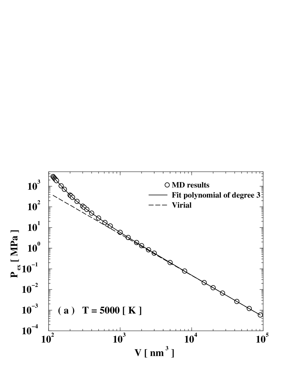
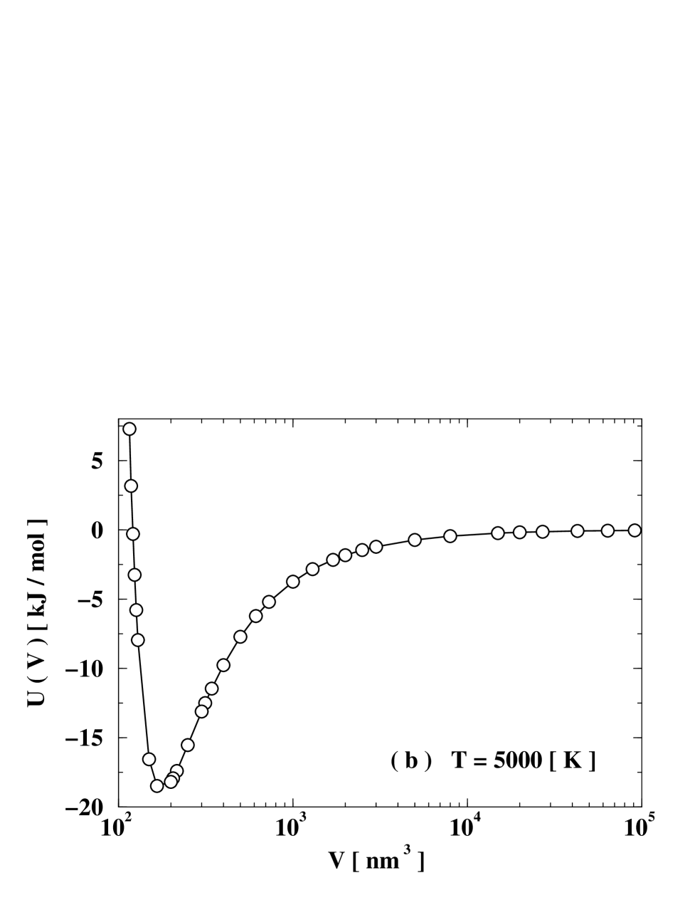
FIG. 2.: (a) Excess pressure at $T=5000$ K as a function of volume. The open circles are the MD results. The dashed line is the the first term of the virial expansion to the excess pressure; the solid line is a third order polynomial fit to the entire set of data. (b) Potential energy at $T=5000$ K as a function of volume.

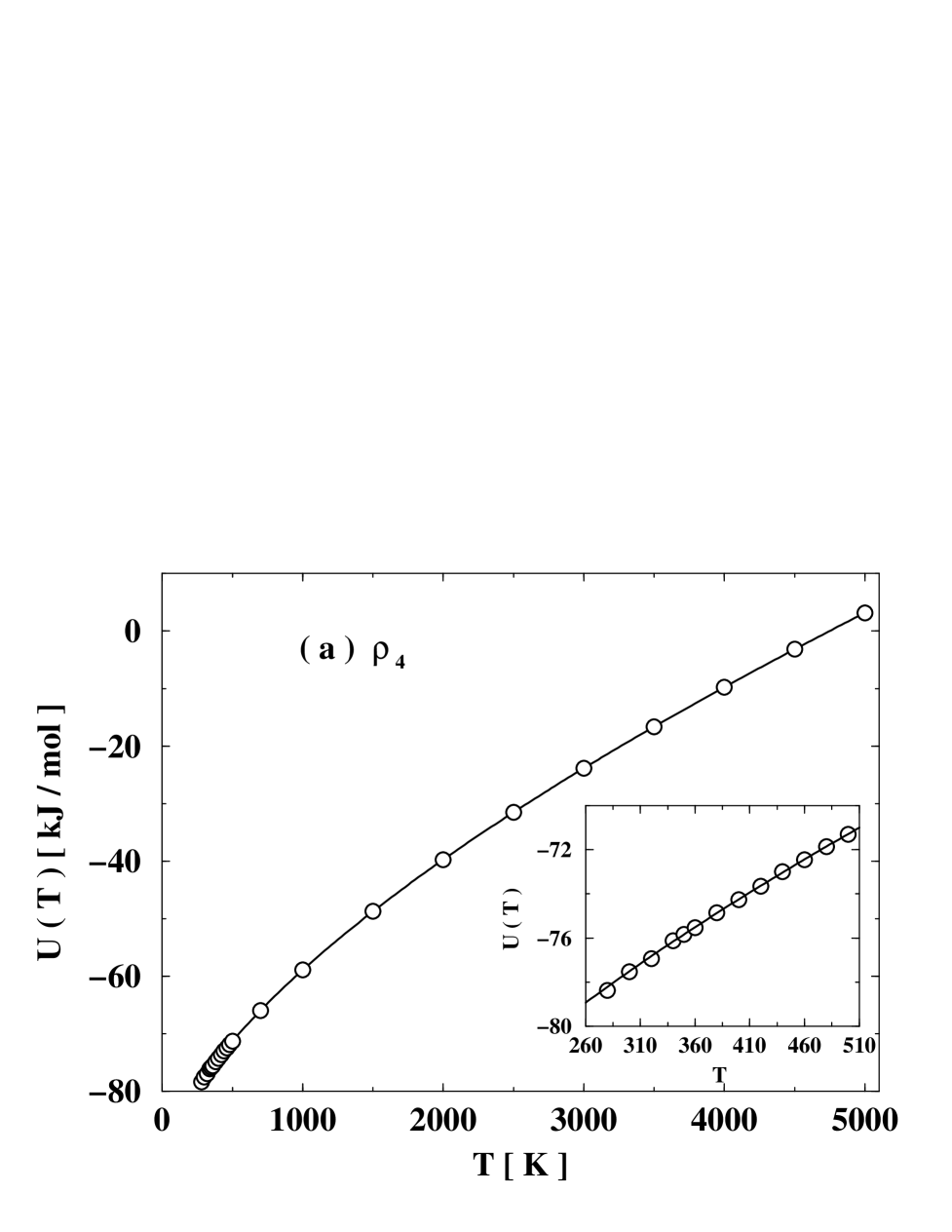
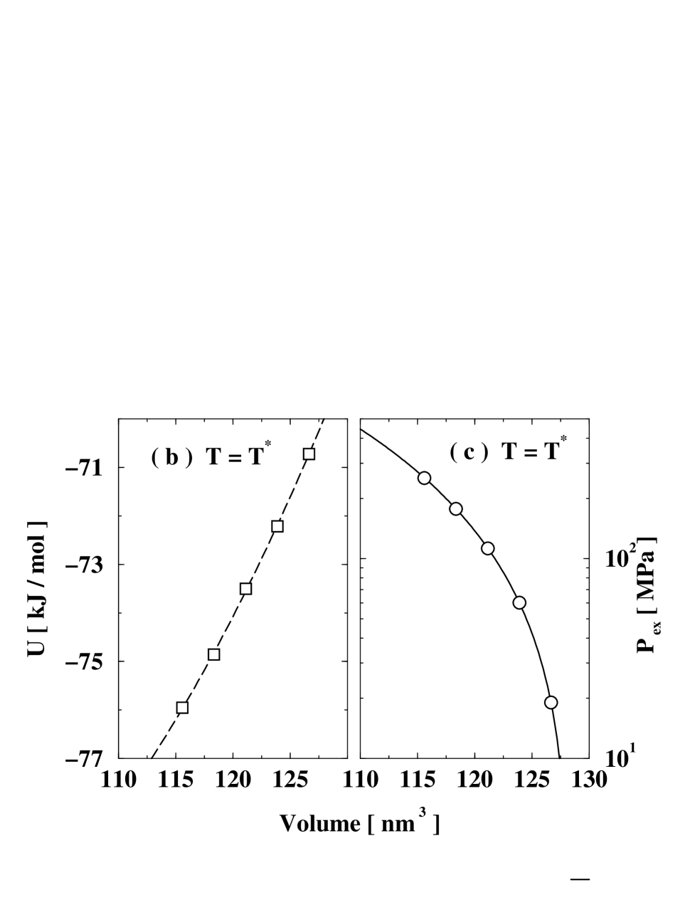
FIG. 3.: (a) Integration Step 2. Potential energy (open circles) at the density $\rho_{4}$ in the entire temperature range considered; the solid line is the fit of the data to Eq. (23). The inset shows the lowest temperatures region in order to stress the accuracy of the fit. (b) and (c) Integration Step 3. Potential energy (b) and pressure (c).

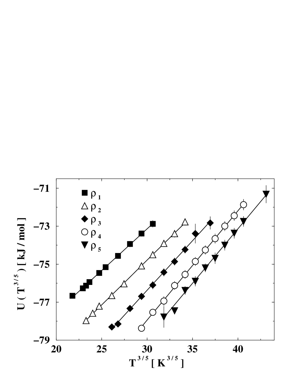
FIG. 4.: Potential energies at the different densities as a function of $T^{3/5}$. The straight solid lines show the validity of the Rosenfeld-Tarazona law Eq. (29).

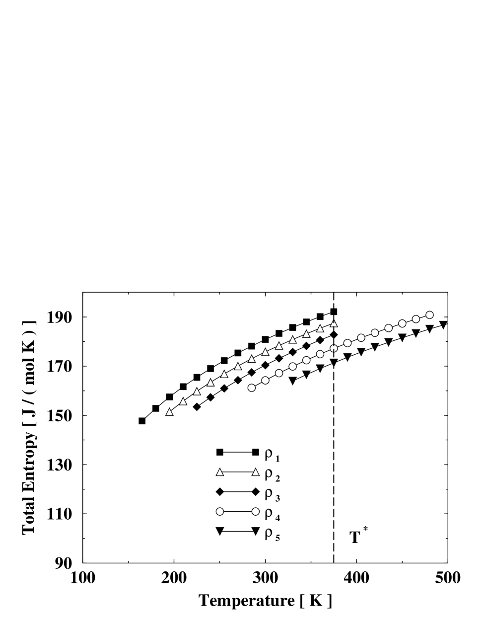
FIG. 5.: Temperature dependence of the total entropy as calculated by thermodynamic integration from the ideal gas reference state. Only points in the temperature range where MD measurements have been performed are shown. The reference temperature $T^{*}=380$ K is also shown (dashed line).

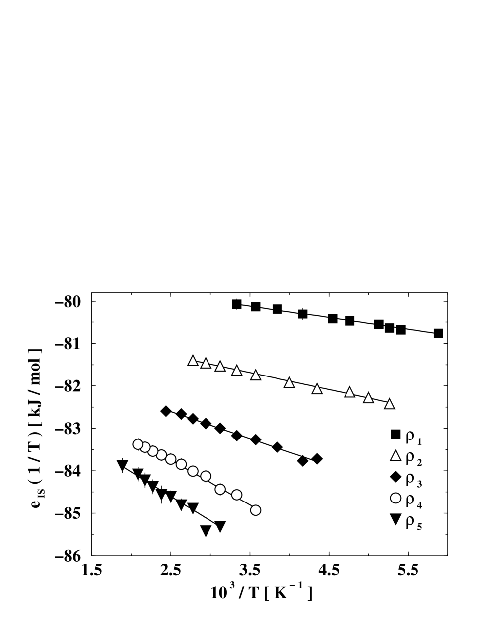
FIG. 6.: Energies of the inherent structures at the different densities as a function of $1/T$. The straight lines confirm the validity of Eq. (30) in the entire temperature range considered.

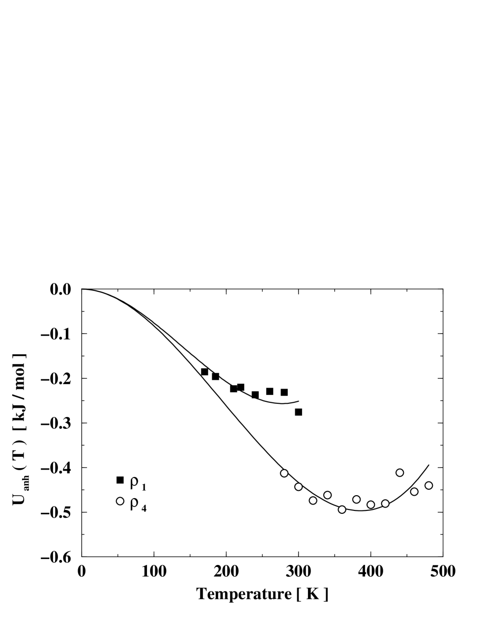
FIG. 7.: Anharmonic contributions to the energies, at the two indicated densities, together with the appropriate cubic fit Eq. (31). This contribution is integrated to directly calculate the anharmonic contribution to the vibrational entropy.

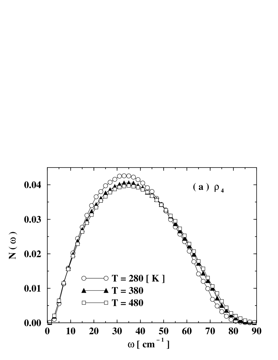
FIG. 8.: (a) Density of states at fixed density $\rho_{4}$ at the three indicated temperatures. This quantity is the histogram of the square root of the eigenvalues of the Hessian calculated for the inherent structures. (b) Density dependence of the density of state at fixed temperature $T=320$ K. The dashed line indicates the isosbestic frequency $\omega^{*}\approx 44$ cm^-1 at which all the curves intersect. The relevance of this feature is discussed in the text.

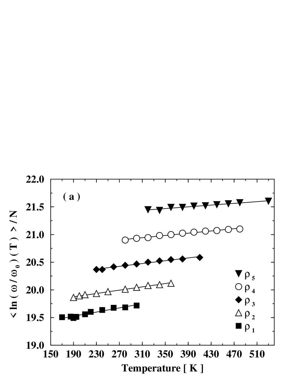
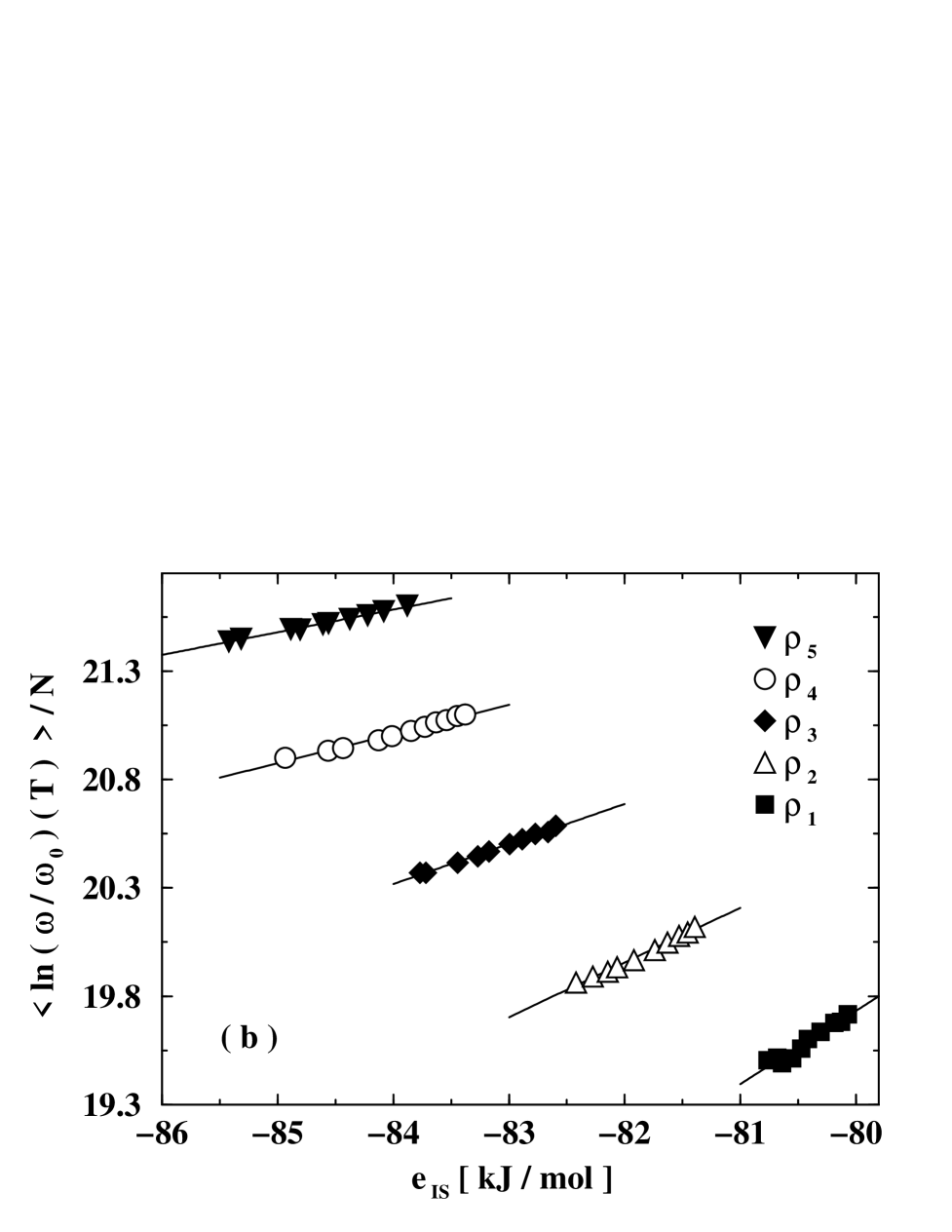
FIG. 9.: (a) Temperature dependence of the average basin curvatures $N^{-1}\sum_{k=1}^{6N-3}\log(\omega_{k}/\omega_{o})$; this quantity, being a sum of logarithms, is very sensitive to the spectrum tails. $\omega_{o}=1$ cm^-1 sets the frequency scale. (b) Relation between the energy of the inherent structures and the average basin curvatures. The straight lines confirm the correlation between shape and depth of the inherent structures accessed by the system.

FIG. 10.: Main panel: Harmonic contribution to the vibrational entropy as calculated from the eigenvalues of the Hessian for the inherent structures. Inset: Anharmonic contribution to the vibrational entropy as calculated by integration of the anharmonic contribution to the potential energy, as discussed in the text.

FIG. 11.: Volume and temperature dependence of the configurational entropy $S_{c}$ calculated as the difference between the total and the vibrational entropy. Solid lines are interpolations of the calculated points to Eq. (34).

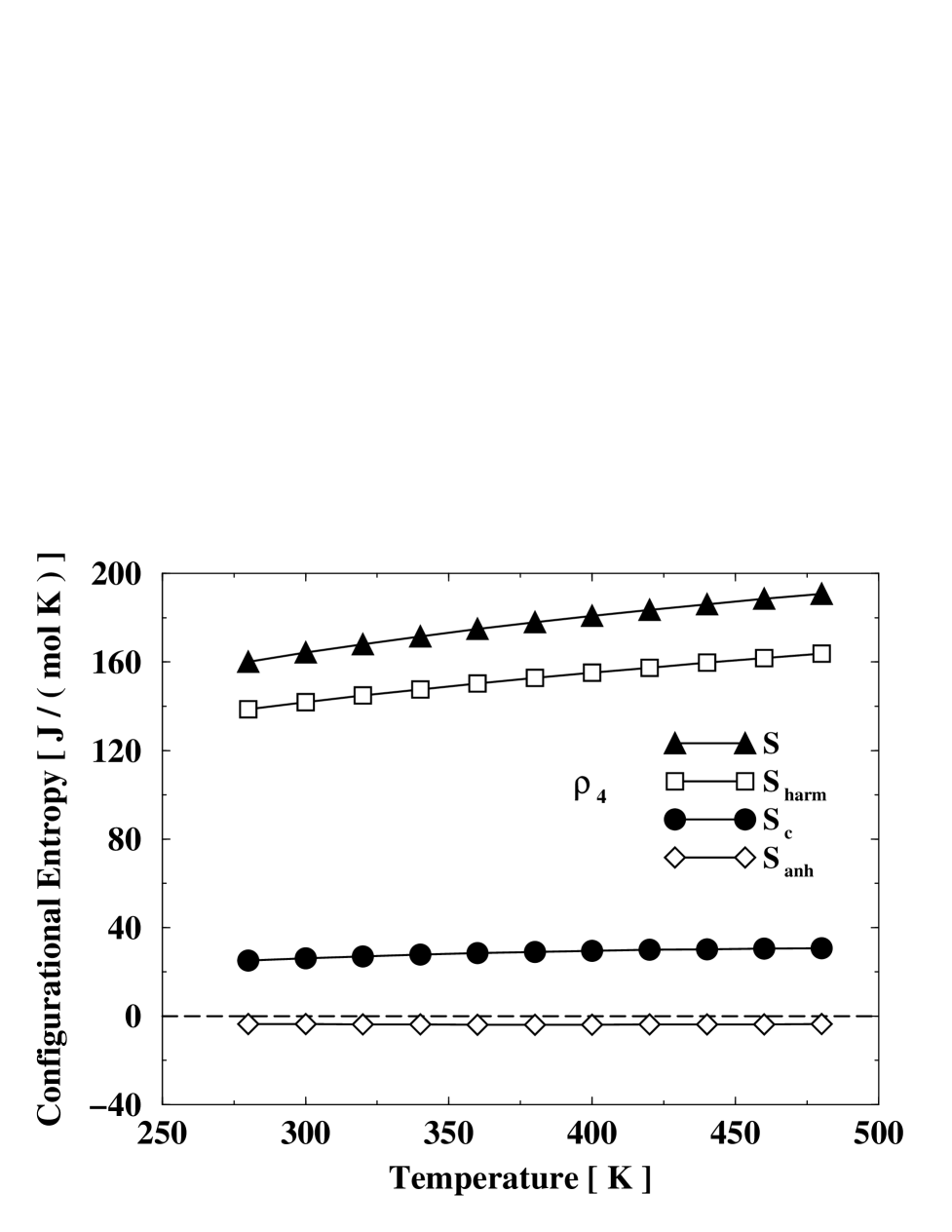
FIG. 12.: Temperature dependence of the different contributions to the total entropy (closed triangles) at the fixed selected density $\rho_{4}$: harmonic (open squares), configurational entropy (closed circles) and anharmonic (open diamonds).

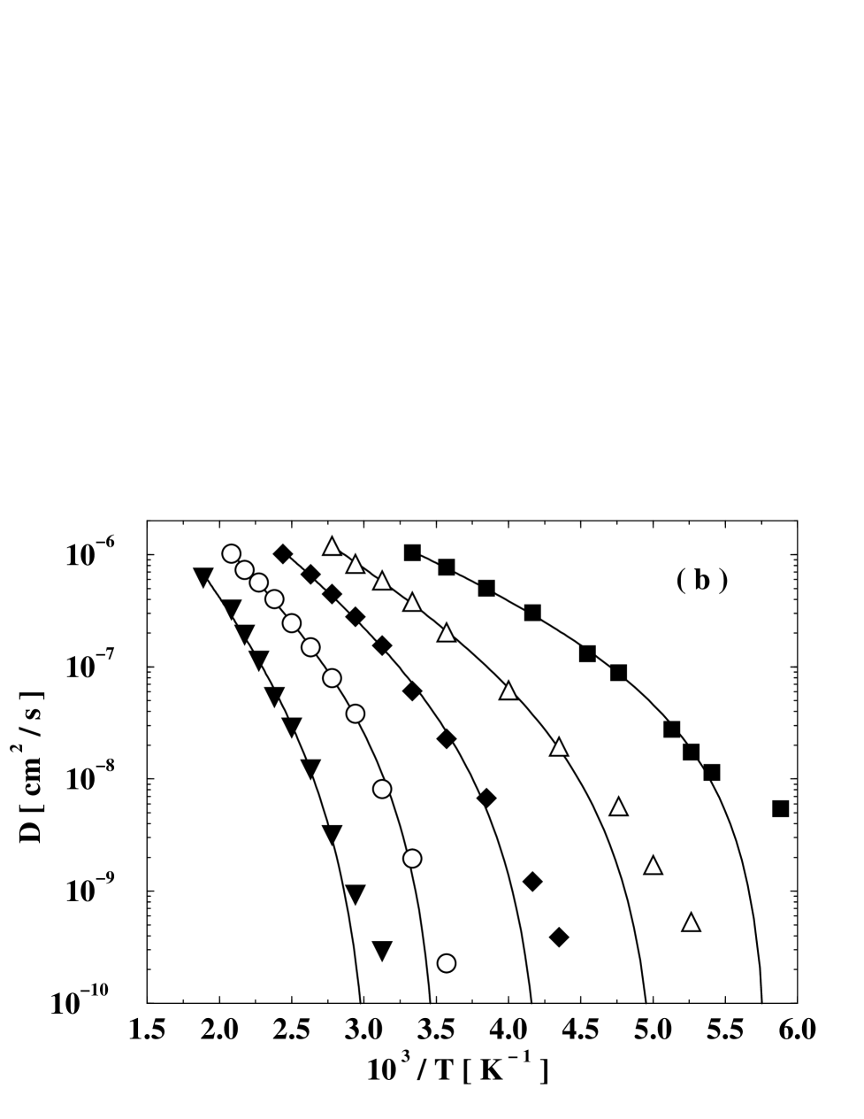
FIG. 13.: Diffusion constants together with the corresponding power law fits (solid lines) predicted by the MCT. The breakdown of this prediction and the crossover to an activated dynamics is evident. See text for a discussion of this point. (a) As a function of temperature. (b) As a function of the inverse temperature in order to stress the exponential dependence at the lowest temperatures.

FIG. 14.: MCT parameters as calculated from the diffusion constants. Main panel: Critical temperature $T_{c}(V)$ (open circles) together with the value calculated in Ref. [42] (closed circle). The dashed line is only a guide for the eye. Inset: Power law exponent $\gamma(V)$.

FIG. 15.: Test of the Adam-Gibbs relation $\log D(T)\propto(1/TS_{c})$ for five different densities. Note that this linear relation holds both above and below the estimated critical temperatures $T_{c}$.

REFERENCES

- [1] P. G. Debenedetti, and F. H. Stillinger, Nature (London) 410, 259 (2001).
- [2] M. Mézard, in More is different, M. P. Ong and R. N. Bhatt eds., Princeton University Press, Princeton, 2001; preprint cond-mat/0110363.
- [3] G. Tarjus, and D. Kivelson, preprint cond-mat/0003368.
- [4] P. G. Debenedetti, Metastable liquids, (Princeton University Press, Princeton, 1997).
- [5] G. Q. Shen, J. Toulouse, S. Beaufils, B. Bonello, Y. H. Hwang, P. Finkel, J. Hernandez, M. Bertault, M. Maglione, C. Ecolivet, and H. Z. Cummins, Phys. Rev. E 62, 783 (2000).
- [6] H. Z. Cummins, J. Phys. Condens. Matter 11, A95 (1999).
- [7] W. Götze, J. Phys. Condens.Matter 11, A1 (1999).
- [8] C. A. Angell, Science 267, 1924 (1995).
- [9] R. Torre, P. Bartolini, and R. M. Pick, Phys. Rev. E 57, 1912 (1998); A. Taschin, R. Torre, M. A. Ricci, M. Sampoli, C. Dreyfus and R. M. Pick, Europhys. Lett. 56, 407 (2001).
- [10] K. Binder et al., in Complex Behaviour of Glassy Systems, M. Rubi and C. Perez-Vicente Eds. (Springer Verlag, Berlin, 1997).
- [11] W. Götze, in Liquids, Freezing and the Glass Transition, edited by J. P. Hansen, D. Levesque and J. Zinn-Justin (North-Holland, Amsterdam, 1991); W. Götze and L. Sjörgen, Rep. Prog. Phys. 55, 241 (1992); W. Götze, J. Phys.: Condensed Matter, 11, A1 (1999).
- [12] R. Schilling, in Disorder Effects on Relaxational Processes edited by A. Richert and A. Blumen (Springer Verlag, 1994); W. Kob, in Experimental and Theoretical Approaches to Supercooled Liquids: Advances and Novel Applications edited by J. Fourkas et al. (ACS Books, Washington, 1997).
- [13] M. Mézard and G. Parisi, Phys. Rev. Lett. 82, 747 (1999); M. Mézard and G. Parisi, J. Phys.: Condens. Matter 12, 6655 (2000).
- [14] X. Xia, P. G. Wolynes, Phys. Rev. Lett. 86, 5526 (2001).
- [15] R. Speedy, J. Phys. Condens. Matter 10, 4185 (1998); ibid. 9, 8591 (1997); ibid. 8, 10907 (1996).
- [16] G. Hinze, D. Brace, S. D. Gottke, and M. D. Fayer, Phys. Rev. Lett. 84, 2437 (2000).
- [17] M. Kiebel, E. Bartsch, O. Debus, F. Fujara, W. Petry, and H. Sillescu, Phys. Rev. B 45, 10301 (1992); A. Tölle, H. Schober, J. Wuttke, and F. Fujara, Phys. Rev. E 56, 809 (1997); A. Tölle, H. Schober, J. Wuttke, O. G. Randl, and F. Fujara, Phys. Rev. Lett. 80, 2374 (1998).
- [18] J. Gapinski, W. Steffen, A. Patkowski, J. Chem. Phys. 110, 2312 (1999); A. Aouadi, C. Dreyfus, M. Massot, J. Chem. Phys. 112, 9860 (2000).
- [19] K. L. Ngai, J. Chem. Phys. 110, 10576 (1999); R. Casalini, K. L. Ngai, C. M. Roland, J. Chem. Phys. 112, 5181 (2000); J. Wuttke, M. Ohl, M. Goldammer, S. Roth, U. Schneider, P. Lunkenheimer, R. Kahn, B. Rufflé, R. Lechner, and M. A. Berg, Phys. Rev. E 61, 2730 (2000); M. Goldammer, C. Losert, J. Wuttke, W. Petry, F. Terki, H. Schober, and P. Lunkenheimer, Phys. Rev. E 64, 021303 (2001).
- [20] T. Gleim, W. Kob, and K. Binder, Phys. Rev. Lett. 81, 4404 (1998).
- [21] L. Fabbian, A. Latz, R. Schilling, F. Sciortino, P. Tartaglia, and C. Theis, Phys. Rev. E. 60, 5768 (1999); ibid. 62, 2388 (2000); C. Theis, F. Sciortino, A. Latz, R. Schilling, and P. Tartaglia, Phys. Rev. E. 62, 1856 (2000).
- [22] F. Sciortino and W. Kob, Phys. Rev. Lett. 86, 648 (2001).
- [23] F. H. Stillinger, and T. A. Weber, Phys. Rev. A 25, 978 (1982); Science 225, 983 (1984); F. H. Stillinger, ibid. 267, 1935 (1995).
- [24] T. B. Schrøder, S. Sastry, J. C. Dyre, and S. C. Glotzer, J. Chem. Phys. 112, 9834 (2000).
- [25] H. Fynewever, D. Perera, P. Harrowell, J. Phys. Condens. Mat. 12, A399 (2000).
- [26] S. Sastry, J. Phys.: Condens. Matter 12, 6515 (2000).
- [27] S. Sastry, Nature (London) 409, 164 (2001).
- [28] F. W. Starr, S. Sastry, E. La Nave, A. Scala, H. E. Stanley, and F. Sciortino, Phys. Rev. E 63, 041201 (2001).
- [29] A. Heuer, Phys. Rev. Lett. 78, 4051 (1997); S. Büchner, and A. Heuer, Phys. Rev. E 60, 6507 (1999).
- [30] I. Saika-Voivod, P. H. Poole, and F. Sciortino, Nature (London) 412, 514 (2001).
- [31] F. Sciortino, W. Kob, and P. Tartaglia, Phys. Rev. Lett. 83, 3214 (1999)
- [32] A. Scala, F. W. Starr, E. La Nave, F. Sciortino, and H. E. Stanley, Nature (London) 406, 166 (2000).
- [33] R. J. Speedy, J. Chem. Phys. 114, 9069 (2001).
- [34] B. Coluzzi, G. Parisi, and P. Verrocchio, Phys. Rev. Lett. 84, 306(2000); B. Coluzzi and P. Verrocchio, preprint cond-mat/0108464; B. Coluzzi, M. Mézard, G. Parisi, and P. Verrocchio, J. Chem. Phys. 111, 9039 (1999); B. Coluzzi, G. Parisi, and P. Verrocchio, J. Chem. Phys. 112, 2933 (2000).
- [35] A. Crisanti, and F. Ritort, preprint cond-mat/0110259
- [36] G. Adam, and J. H. Gibbs, J. Chem. Phys. 43, 139 (1965).
- [37] W. Kob, F. Sciortino, and P. Tartaglia, Europhys. Lett. 49, 590 (2000)
- [38] S. Mossa, G. Ruocco, F. Sciortino, and P. Tartaglia, preprint cond-mat/0107142.
- [39] A. Scala and F. Sciortino, preprint cond-mat/0106573.
- [40] F. Sciortino and P. Tartaglia, J. Phys. Condensed Matter 13 9127 (2001).
- [41] G. Wahnström and L. J. Lewis, Physica A 201, 150 (1993); L. J. Lewis and G. Wahnström, Solid State Comm. 86, 295 (1993); J. Non-Crystalline Solids 172-174, 69 (1994); Phys. Rev. E 50, 3865 (1994); G. Wahnström and L. J. Lewis, Prog. Theor. Phys. Suppl. 126, 261 (1997).
- [42] A. Rinaldi, F. Sciortino, and P. Tartaglia, Phys. Rev. E 63, 061210 (2001).
- [43] S. Mossa, R. Di Leonardo, G. Ruocco, and M. Sampoli, Phys. Rev. E 62, 612 (2000); S. Mossa, G. Ruocco, and M. Sampoli, ibid. 64, 021511 (2001); S. Mossa, G. Monaco, and G. Ruocco, preprint cond-mat/0104265; S. Mossa, G. Monaco, G. Ruocco, M. Sampoli, and F. Sette, J. Chem. Phys. (in press), preprint cond-mat/0104129.
- [44] F. Sciortino, W. Kob, and P. Tartaglia, J. Phys.: Condens. Matter 12, 1 (2000).
- [45] Y. Rosenfeld, and P. Tarazona, Mol. Phys. 95, 141 (1998).
- [46] G. E. Walrafen, M. S. Hokmabadi, and W. H. Yang, J. Chem. Phys. 85, 6964 (1986). See also P. Benassi, V. Mazzacurati, M. Nardone, M. A. Ricci, G. Ruocco, and G. Signorelli, J. Chem. Phys. 88, 4553 (1988).
- [47] C. A. Angell, B. E. Richards, and V. Velikov, J. Phys. Condensed Matter 11, A75 (1999).
- [48] F. Sciortino, and P. Tartaglia, Phys. Rev. Lett. 86, 107 (2001).
- [49] L. M. Martinez, and C. A. Angell, Nature (London) 410, 667 (2001).
- [50] F. H. Stillinger, J. Phys. Chem. B 102, 2807 (1998).
- [51] R. Richert, and C. A. Angell, J. Chem. Phys. 108, 9016 (1998).
- [52] M. Dzugutov, Nature (London) 381, 137 (1996); M. Dzugutov, J. Phys. Condens. Matter 11, A253 (1999).
- [53] M. Schulz, Phys. Rev. B 57, 11319 (1998).
- [54] T. Keyes, J. Phys. Chem. 101, 2921 (1997).
- [55] F. Sciortino, and P. Tartaglia, Phys. Rev. Lett. 78, 2385 (1997).
- [56] C. Donati, F. Sciortino and P. Tartaglia, Phys. Rev. Lett. 85, 1464 (2000).
- [57] E. La Nave, A. Scala, F. W. Starr, F. Sciortino, and H. E. Stanley, Phys. Rev. Lett. 84, 4605 (2000).
- [58] E. La Nave, A. Scala, F. W. Starr, H. E. Stanley, and F. Sciortino, Phys. Rev. E 64, 036102 (2001).
- [59] E. La Nave, H. E. Stanley, and F. Sciortino, Phys. Rev. Lett. (in press), preprint cond-mat/0108546.
- [60] J. E. Mayer, and M. G. Mayer, Statistical Mechanics, (John Wiley & Sons, New York, 1963).