[

Many-body $GW$ Calculations of Ground-State Properties: Quasi-2D Electron Systems and van der Waals Forces

Abstract

We present $GW$ many-body results for ground-state properties of two simple but very distinct families of inhomogenous systems in which traditional implementations of density-functional theory (DFT) fail drastically. The $GW$ approach gives notably better results than the well-known random-phase approximation, at a similar computational cost. These results establish $GW$ as an superior alternative to standard DFT schemes without the expensive numerical effort required by quantum Monte Carlo simulations.

]

Ab initio many-body-theory (MBT) methods, particularly those based on Hedin’s GW approximation [1], have been used extensively during the last decade to calculate excited-state properties of electron systems in solid-state physics [2]. In addition, there is a recent and increasing interest in the application of such methods to obtain ground-state properties [3, 4, 5, 6, 7, 8, 9, 10]. In MBT, electron-electron correlations are taken into account directly without resorting to the mean-field density-based approximations used in routine implementations of Density Functional Theory (DFT) [11], thus providing a more microscopic description of the interacting many-electron problem.

Modern MBT calculations use efficient algorithms for the evaluation of MBT quantities [such as the dielectric function $\hat{\epsilon}\left(\omega\right)$, the self-energy operator $\hat{\Sigma}\left(\omega\right)$, and the one-particle Green function $\hat{G}\left(\omega\right)$] required in the study of excited-state properties of real materials [12, 13]. The application of these techniques to the calculation of ground-state properties, such as the density or the total energy, opens the appealing possibility of treating all the electronic properties in the same fashion. Although more expensive than DFT, these MBT methods do not require the demanding computational effort of quantum Monte Carlo simulations [14]. Nonetheless, ground-state calculations based on MBT must be painstakingly assessed. First, approximations that have proved successful for spectral properties might not necessarily be good methods for structural properties. Second, the energies and lifetimes of quasiparticles are mainly determined by the pole structure of $\hat{G}\left(\omega\right)$, while ground-state properties emerge from a multidimensional integration of $\hat{G}\left(\omega\right)$. As a consequence, features that can be safely ignored in the determination of quasiparticle properties, like the high-frequency behavior or high-energy-transfer matrix elements, play an important role if we want to calculate, for instance, the ground-state energy. The development of general-purpose procedures requires a careful study of the optimal treatment of these points.

In this Letter we present nonselfconsistent (in the sense described below) GW calculations for the ground-state properties of two families of simple inhomogeneous systems: the quasi-two-dimensional (2D) electron gas and a pair of interacting jellium slabs. These provide a suitable test cases for an extensive assessment of the performance of $GW$-MBT ground-state calculations. First, despite the simplicity of these systems, LDA and GGA fail to describe them properly. For the quasi-2D gas, the high inhomogeneity of the density profile along the confining direction is clearly beyond the scope of local or semilocal approaches [15]. The situation is quite different if we consider interacting jellium slabs. In the limit of large separation, in which the densities of each subsystem do not overlap, dispersion or van der Waals (vdW) forces are evident. These forces are due to long-ranged Coulomb correlations and, hence, cannot be described at all by the LDA or GGA [4, 16]. As shown below, even nonlocal DFT prescriptions for the XC energy, such as the weighted density approximation (WDA) [17], are unable to reproduce such forces. On the other hand, these systems exhibit translational invariance along the xy plane, thus reducing significantly the number of independent variables needed to describe the spatial dependence of all the operators, assisting the production of the highly-converged test calculations required here.

In Hedin’s $GW$ framework, the self-energy $\hat{\Sigma}$ of a system of $N$ electrons under an external potential $v_{{\rm ext}}\left({\bf r}\right)$ is approximated by

$$\Sigma\left(1,2\right)=iG\left(1,2^{+}\right)W\left(1,2\right),$$ (1)

where the labels 1 and 2 symbolize space-time coordinates. $\hat{W}$ is the screened Coulomb potential, which is exactly related to the bare Coulomb potential $\hat{w}$ and the polarizability $\hat{P}$ by $\hat{W}\left(\omega\right)=\hat{w}+\hat{w}\hat{P}\left(\omega\right)\hat{W}\left(\omega\right)=\hat{\epsilon}^{-1}\left(\omega\right)\hat{w}$ (the usual matrix operations are implied). Under the $GW$ approach, the polarizability is given by $P\left(1,2\right)=-2iG\left(1,2\right)G\left(2,1^{+}\right)$. Finally, $\hat{\Sigma}$ and $\hat{G}$ are linked through the Dyson equation $\hat{G}^{-1}\left(\omega\right)=\omega-[\hat{t}+\hat{v}_{{\rm el}}+\hat{\Sigma}\left(\omega\right)]$, with $\hat{t}$ the one-electron kinetic energy, and $v_{{\rm el}}\left({\bf r}\right)$ the classical electrostatic potential [the sum of $v_{{\rm ext}}\left({\bf r}\right)$ and the Hartree interaction potential]. This set of equations defines a selfconsistent problem, but routine $GW$ calculations concerned with the quasiparticle properties do not attempt selfconsistency: when evaluating $\hat{\Sigma}$, the interacting Green function $\hat{G}$ is generally substituted by that corresponding to the noninteracting Kohn-Sham (KS) system under the LDA (or GGA) approximation.

It is well known that full selfconsistency implies a worsening of the description of spectral properties [18]. However, for the 3D [5, 10] and 2D [10] homogeneous electron gases, the total energy arising from $\hat{G}$ by using the Galitskii-Migdal formula of MBT [19] fits the (essentially exact) QMC values extremely well if $\hat{G}$ is obtained selfconsistently. Nonetheless, at the nonselfconsistent level (which we will call $G_{0}W_{0}$) the exact exchange energy is already built in and, at the same time, correlation effects beyond the random-phase approximation (RPA) are taken into account, as reflected in good total energies and very good total energy differences [5, 10] for these homogeneous systems. Since the relevant quantity for structural properties is the total energy difference, $G_{0}W_{0}$ (and even, in some cases, RPA [20]) is likely to fulfill a useful role. The known particle-number violation under the $G_{0}W_{0}$ approximation [21], while non-zero, is so small that it can be ignored in practical applications [22].

All the calculations reported in this Letter are done as follows. First, we perform a standard LDA-KS calculation, in which, owing to the translational invariance along the $xy$ plane, the KS orbitals are organized into subbands. That is, each KS state is given by $\phi_{n{\bf k}}\left({\bf r}\right)=\psi_{n}\left(z\right)e^{i{\bf k}\cdot\mbox{\boldmath$\rho$}}/\sqrt{2\pi}$, where ${\bf k}=\left(k_{x},k_{y}\right)$ and $\mbox{\boldmath$\rho$}=\left(x,y\right)$ denote the two-dimensional momentum and position in the $xy$-plane. Then, the noninteracting polarizability $P_{0}\left(1,2\right)=-2iG_{0}\left(1,2\right)G_{0}\left(2,1^{+}\right)$ is calculated at imaginary frequencies using the expression

$$P_{0}\left(z,z^{\prime},k;{\rm i}\omega\right)=\sum_{n=1}^{N_{{\rm occ}}}\sum_{m=1}^{\infty}S_{nmk}\left({\rm i}\omega\right)\gamma_{nm}\left(z\right)\gamma_{nm}\left(z^{\prime}\right)$$ (2)

Here, $N_{{\rm occ}}$ is the number of occupied KS subbands, $\gamma_{nm}\left(z\right)=\psi_{n}\left(z\right)\psi_{m}\left(z\right)$, and the coefficients $S_{nmk}\left({\rm i}\omega\right)$ admit a fully analytical expression [9, 23]. $P_{0}\left({\rm i}\omega\right)$ could be also calculated fully numerically [13] but due to the high symmetry of the system, the present method is more efficient. The infinite sum in Eq. 2 is truncated at a certain value $N_{{\rm B}}$, which acts as a convergence parameter.

The next step is the inversion of the RPA dielectric function $\hat{\epsilon}_{0}\left({\rm i}\omega\right)=\hat{1}-\hat{w}\hat{P}_{0}\left({\rm i}\omega\right)$ and the evaluation of $\hat{W}_{0}\left({\rm i}\omega\right)=\hat{\epsilon}_{0}^{-1}\left({\rm i}\omega\right)\hat{w}$. This can be done in a double cosine basis representation [9, 22], but the high inhomogeneity of the systems along the $z$ direction suggests a different method based on Ref. [12]. Note that the polarizability spans a Hilbert space made up by the product states $\gamma_{nm}$. Obviously, the set $\left\{\gamma_{nm}\right\}$ has a large number of linear dependences which can be eliminated using a standard Gramm-Schmidt procedure, so obtaining an optimized basis set ${\cal B}_{{\rm op}}=\left\{\zeta_{\alpha}\left(z\right)\right\}$. In all the cases here studied, $N_{{\rm op}}=N_{{\rm B}}+N_{{\rm occ}}-1$ $\zeta$-functions ensure an almost perfect representation (with a relative error less than $10^{-4}$) of all the product states $\gamma_{nm}$. Hence, $P_{0}\left(z,z^{\prime},k;{\rm i}\omega\right)=\sum_{\alpha,\beta}\zeta_{\alpha}\left(z\right)P_{0}\left(k,{\rm i}\omega\right)_{\alpha\beta}\zeta_{\beta}\left(z^{\prime}\right)$, where the matrix elements $P_{0}\left(k,{\rm i}\omega\right)_{\alpha\beta}$ can be immediately obtained from $S_{nmk}$ and the scalar products $\left\langle\gamma_{nm},\zeta_{\alpha}\right\rangle$. Then, we calculate the representation $w\left(k\right)_{\alpha\beta}$ of the bare Coulomb potential, and the matrix elements $W\left(k,{\rm i}\omega\right)_{\alpha\beta}$ of the screened Coulomb potential are easily obtained by a matrix inversion for each value of $k$. Well converged results are typically obtained with $N_{{\rm B}}\simeq 80$ subbands, although for quasi-2D systems $N_{{\rm B}}$ is significantly less. RPA correlation energies, where required, can be straightforwardly obtained in this representation.

The real-space representation of $\hat{W}_{0}$ is given by the expansion

$$W_{0}\left(z,z^{\prime},;{\rm i}\tau\right) = {\rm i}\sum_{\alpha,\beta,{\bf k}}\int\frac{d\omega}{2\pi}e^{{\rm i}\left(\omega\tau+{\bf k}\cdot\mbox{\boldmath$\rho$}\right)}$$

$$\times\zeta_{\alpha}\left(z\right)\zeta_{\beta}\left(z^{\prime}\right)W\left(k,{\rm i}\omega\right)_{\alpha\beta}\;,$$

where $\sum_{{\bf k}}=\left(2\pi\right)^{-2}\int d{\bf k}$, whereas the KS Green function $G_{0}\left(z,z^{\prime},\rho;{\rm i}\tau\right)$ is calculated directly from the KS eigenstates [13]. By using (1) we readily get the self-energy operator in real space and imaginary time and, eventually, its representation $\Sigma\left(k,{\rm i}\tau\right)_{nm}$ in the KS basis set. We use typically 100 (or fewer) $\tau/\omega$ points in a Gauss-Legendre grid with $\omega_{\max}\simeq 80\Delta_{c}$ ($\Delta_{c}$ is the width of the conduction band), and 100-150 $\rho/k$ points with $k_{\max}^{2}/2\simeq\omega_{\max}$. It is important to emphasize that the asymptotic time and frequency tails of all the operators must be treated analytically to ensure smooth and rapid convergence.

In the imaginary-time/frequency representation $\hat{\Sigma}\left(\mu+{\rm i}\omega\right)=-{\rm i}\int d\tau\,\hat{\Sigma}\left({\rm i}\tau\right)e^{-{\rm i}\omega\tau}$, with $\mu$ the interacting chemical potential. Hence, the Green function at imaginary frequencies is the solution of the Dyson equation

$$\hat{G}^{-1}\left(\mu+{\rm i}\omega\right)=\mu+{\rm i}\omega-\left[\hat{h}_{{\rm KS}}+\hat{\Sigma}\left(\mu+{\rm i}\omega\right)-\hat{v}_{{\rm XC}}\right]$$ (3)

with $\hat{h}_{{\rm KS}}=\hat{t}+\hat{v}_{{\rm S}}$ the KS-LDA hamiltonian and $v_{{\rm XC}}\left({\bf r}\right)$ the LDA-XC potential. $\hat{G}$ is calculated in the KS representation $G\left(k,{\rm i}\omega\right)_{nm}$, with $\mu$ previously obtained by diagonalizing the quasiparticle hamiltonian at ${\rm i}\omega=0$, $\hat{h}_{{\rm QP}}\left(\mu\right)=\hat{h}_{{\rm KS}}+\hat{\Sigma}\left(\mu\right)-\hat{v}_{{\rm XC}}$, and by imposing that the volume enclosed by the interacting Fermi surface equals the KS value. A small term $\delta v\left({\bf r}\right)$, accounting for the change in the Hartree potential due to the differences between the $G_{0}W_{0}$ and LDA densities, should be included into (3) and $\hat{h}_{{\rm QP}}$. However, this term induces an imperceptible change in the shape of $\hat{G}$, and it has a negligible influence on the ground-state properties.

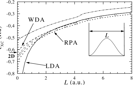
FIG. 1.: XC energy per particle for thin confined jellium slabs of fixed 2D density $n^{{\rm 2D}}=3/4\pi$ as a function of their thickness $L$. Lines: LDA, WDA, and RPA; circles: $G_{0}W_{0}$. The exchange energy (dash-dotted line) has been included as a reference. Note the effect due to the filling of a second subband at $L\simeq 4.2a_{0}$, which is especially evident in $\varepsilon_{{\rm X}}$. The arrow indicates the QMC value for the 2D limit.

The electron density and energy are given, respectively, by $n\left({\bf r}\right)=\pi^{-1}\oint d\omega\,G\left({\bf r,r};{\rm i}\omega\right)$ and $E=E_{{\rm el}}+\pi^{-1}\,{\rm tr}\oint d\omega[\hat{t}+\frac{1}{2}\hat{\Sigma}\left({\rm i}\omega\right)]\hat{G}\left({\rm i}\omega\right)$, where $E_{{\rm el}}$ is the classical electrostatic energy [which can be obtained from $n\left({\bf r}\right)$], and tr symbols the spatial trace. Owing to the symmetry of our model systems (the generalization to arbitrary geometries is straightforward), we can write $n\left(z\right)=n_{0}\left(z\right)+\delta n\left(z\right)=n_{0}\left(z\right)+\sum_{n,{\bf k}}\left|\psi_{n}\left(z\right)\right|^{2}\delta f_{nk}$, $n_{0}\left(z\right)$ being the LDA density, and

$$\delta f_{nk}=\int\frac{d\omega}{\pi}\left[G\left(k,\mu+{\rm i}\omega\right)_{nn}-G_{0}\left(k,\mu_{0}+{\rm i}\omega\right)_{nn}\right]\,,$$ (4)

($\mu_{0}$ is the LDA chemical potential). On the other hand, the exchange energy per surface unit is given directly by $E_{{\rm X}}/S=\frac{1}{2}\sum_{n,{\bf k}}\,f_{nk}\Sigma_{{\rm X}}\left(k\right)_{nn}$, where $\hat{\Sigma}_{{\rm X}}$ is the frequency-independent part of the self-energy $\Sigma_{{\rm X}}\left({\bf r}_{1},{\bf r}_{2}\right)={\rm i}\lim_{\tau\rightarrow 0^{+}}G_{0}\left({\bf r}_{1},{\bf r}_{2};{\rm i}\tau\right)w\left(r_{12}\right)$ (i.e., the Fock operator). Finally, the correlation energy $E_{{\rm C}}$ is written as the sum of its kinetic-energy and electrostatic parts:

$$\frac{T_{{\rm C}}}{S} = \sum_{n,{\bf k}}\varepsilon_{nk}\delta f_{nk}-\int dzv_{{\rm S}}\left(z\right)\delta n\left(z\right)$$ (5)

$$\frac{W_{{\rm C}}}{S} = \sum_{n,{\bf k}}\left[\frac{1}{2}\Sigma_{{\rm X}}\left(k\right)_{nn}\delta f_{nk}+\right.$$ (7)

$$\left.\sum_{m}\int\frac{d\omega}{\pi}\Sigma_{{\rm C}}\left(k,\mu+i\omega\right)_{nm}G\left(k,\mu+i\omega\right)_{mn}\right]$$

where we have included the frequency-dependent part of the self-energy $\hat{\Sigma}_{{\rm C}}\left({\rm i}\omega\right)=\hat{\Sigma}\left({\rm i}\omega\right)-\hat{\Sigma}_{{\rm X}}$. As usual, we suppose that the total electrostatic energy is given correctly by the LDA, since we have checked carefully that the density variation $\delta n\left(z\right)$ causes only minor changes in the electronic energy. We also note that when evaluating $E_{{\rm C}}$ we do not need all the matrix elements of $\hat{\Sigma}$ and $\hat{G}$. In general, full convergence is achieved by performing the sum only over LDA states such that $\varepsilon_{n{\bf k}}\lesssim 6\Delta_{c}$, and this also applies to the resolution of Dyson’s equation. Therefore, the most demanding part of the calculation is the evaluation of $\hat{\epsilon}^{-1}\left({\rm i}\omega\right)$ which, in any case, is required to obtain the RPA correlation energy.

To mimic a quasi-2D electron system, we have taken a thin jellium slab with a background density $\overline{n}=(\frac{4}{3}\pi r_{{\rm s}}^{3})^{-1}$ and width $L$. This slab is bounded by two infinite planar walls, and overall charge neutrality is assumed. We keep the number of particles per unit surface area $n_{{\rm 2D}}=\overline{n}L$ constant, in such a way that the limit $L\rightarrow 0$ corresponds to a 2D homogeneous electron gas (HEG) with density $n_{{\rm 2D}}$. In Fig. 1 we plot, for several values of $L$, the XC energy per particle $\varepsilon_{{\rm XC}}$ given by the LDA, the nonlocal WDA, the RPA, and the $G_{0}W_{0}$ method. As commented previously, the LDA diverges when approaching the 2D limit, whereas the WDA behaves reasonably well, slightly underestimating the absolute value of $\varepsilon_{{\rm XC}}$ in the strict 2D limit. The RPA does not show any pathological behaviour, but it overestimates $\left|\varepsilon_{{\rm XC}}\right|$ by more than 20 mHa/e^- for all configurations. Finally, $G_{0}W_{0}$, whose superiority to the RPA has already been established in the 3D limit,[5, 10] retains this in the transition to the 2D limit. Its performance is similar to that of the WDA for these systems (although the residual error for the 2D gas has the opposite sign). It is important to point out that the RPA and $G_{0}W_{0}$ XC energies obtained by starting from a WDA-KS calculation are indistinguishable from those plotted in Fig. 1. Thus, the specific choice of the KS method seems to be of minor importance when calculating XC energies using MBT.

The study of the interacting energy between two unconfined jellium slabs is of more direct significance, as it has been considered as a benchmark for seamless correlation functionals attempting to describe vdW forces [4, 24]. By varying the distance $d$ between the slabs we cover configurations in which the density profiles of each subsystem overlap (i.e. there is a covalent bond), and situations (when $d\gg 0$) in which there is no such overlap and the only source of bonding is the appearance of vdW forces. In the upper panel of Fig. 2 we plot the XC energy per particle $\varepsilon_{{\rm XC}}\left(d\right)$ as a function of $d$ using the LDA (the WDA gives very similar results), the RPA, and the $G_{0}W_{0}$, for two slabs of width $L=12a_{0}$ and a background density $\overline{n}$ corresponding to $r_{{\rm s}}=3.93$. We can see that the $G_{0}W_{0}$ reduces the RPA error by 60%. In the lower panel we represent the correlation binding energy per particle [defined as $e_{{\rm C}}\left(d\right)=\varepsilon_{{\rm C}}\left(d\right)-\varepsilon_{{\rm C}}\left(\infty\right)$]. First, neither the LDA nor even the nonlocal WDA is able to reproduce the characteristic asymptotic $d^{-2}$ vdW behavior. This behavior is described by the RPA and the $G_{0}W_{0}$, and for both approximations $e_{{\rm C}}\left(d\gg 0\right)$ is very similar (which is not a surprise because such an asymptotic behavior is fully described at the RPA level [4]). For intermediate and small separations, there are slight differences between the RPA and the $G_{0}W_{0}$ but much less important than those appearing when comparing the total correlation energies.

A detail that is worth pointing out is the fact that the error in the absolute $G_{0}W_{0}$ correlation energy is amenable to a LDA-like correction. From the differences, given in Ref. [10], between QMC and $G_{0}W_{0}$ correlation energies for the HEG, we can build a functional $\Delta E_{{\rm C}}=\int d{\bf r}n\left({\bf r}\right)\,\delta\varepsilon_{{\rm C}}\left[n\left({\bf r}\right)\right]$. The absolute $G_{0}W_{0}$ energy corrected in this way is in broad correspondence with the LDA energy, while the binding energy retains its correct $1/d^{2}$ behavior at large $d$ and is little altered for small $d$ (see Fig. 2).

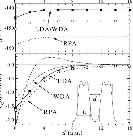
FIG. 2.: Upper panel: XC energy per particle for two jellium slabs as a function of the distance $d$. Lines: LDA, WDA and RPA; circles: $G_{0}W_{0}$; squares: $G_{0}W_{0}$ plus LDA-like correction term. Lower panel: correlation binding energy per particle. The LDA and WDA contributions have been obtained by subtracting the exact exchange energy from the corresponding XC values. The exchange binding energy (dashed-dotted line) has been also included in this panel.

In summary, we have performed $GW$-MBT calculations to evaluate the ground-state energy of inhomogeneous systems. With practically the same cost we have obtained correlation energies beyond the random phase approximation. The importance of a truly ab initio treatment of electron many-body effects is evident in the model systems we have chosen, for which traditional implementations of DFT are completely inaccurate.

The authors thank C.-O. Almbladh, J.E. Alvarellos, U. von Barth, E. Chacón, J. Dobson, B. Holm, P. Rinke, and A. Schindlmayr for many valuable discussions. This work was funded in part by the EU through the NANOPHASE Research Training Network (Contract No. HPRN-CT-2000-00167) and by the Spanish Education Ministry DGESIC grant PB97-1223-C02-02.

REFERENCES

- [1] L. Hedin, Phys. Rev. 139, A796 (1965).
- [2] See, for instance: F. Aryasetiawan and O. Gunnarsson, Rep. Prog. Phys. 61, 237 (1998); W.G. Aulbur, L. Jönsson, and J.W. Wilkins, Solid State Physics 54, 1 (2000).
- [3] M.M. Rieger and R.W. Godby, Phys. Rev. B 58, 1343 (1998).
- [4] J.F. Dobson and J. Wang, Phys. Rev. Lett. 82, 2123 (1999); Phys. Rev. B 62, 10038 (2000).
- [5] B. Holm, Phys. Rev. Lett. 83, 788 (1999).
- [6] C.-O. Almbladh, U. von Barth, and R. van Leeuwen, Int. J. Mod. Phys. B 13, 535 (1999).
- [7] B. Holm and F. Aryasetiawan, Phys. Rev. B 62, 4858 (2000).
- [8] P. Sánchez-Friera and R. W. Godby, Phys. Rev. Lett. 85, 5611 (2000).
- [9] J.M. Pitarke and A.G. Eguiluz, Phys. Rev. B 63, 045116 (2001).
- [10] P. García-González and R.W. Godby, Phys. Rev. B 63, 075112 (2001).
- [11] P. Hohenberg and W. Kohn, Phys. Rev. 136, B864 (1964); W. Kohn and L.J. Sham, ibid. 140, A1133 (1965).
- [12] F. Aryasetiawan and O. Gunnarsson, Phys. Rev. B 49, 16214 (1994).
- [13] H.N. Rojas, R.W. Godby, and R.J. Needs, Phys. Rev. Lett. 74, 1827 (1995); M.M. Rieger et al., Computer Physics Communications 117, 211 (1999); L. Steinbeck et al., ibid. 125, 105 (2000).
- [14] W.M.C. Foulkes et al., Rev. Mod. Phys. 73, 17 (2000).
- [15] Y. Kim et al., Phys. Rev. B 61, 5202 (2000); L. Pollack and J.P. Pedew, J. Phys.: Condens. Matter 12, 1239 (2000); P. García-González, Phys. Rev. B 62, 2321 (2000).
- [16] W. Kohn, Y. Meir, and D.E. Makarov, Phys. Rev. Lett. 80, 4153 (1998).
- [17] O. Gunnarsson, M. Jonson, and B.I. Lundqvist, Phys. Rev. B 20, 3136 (1979); E. Chacón and P. Tarazona, Phys. Rev. B 37, 4013 (1988).
- [18] B. Holm and U. von Barth, Phys. Rev. B 57, 2108 (1998); W.D. Schöne and A.G. Eguiluz, Phys. Rev. Lett. 81, 1662 (1998).
- [19] V.M. Galitskii and A.B. Migdal, Zh. Eksp. Teor. Fiz. 34, 139 (1958) [Sov. Phys. JETP 7, 96 (1958)].
- [20] S. Kurth and J.P. Perdew, Phys. Rev. B 59, 10461 (1999); Z. Yan et al., ibid. 61, 2595 (2000).
- [21] A. Schindlmayr, Phys. Rev. B 56, 3528 (1997).
- [22] A. Schindlmayr, P. García-González, and R.W. Godby, Phys. Rev. B (in press).
- [23] A. G. Eguiluz, Phys. Rev. B 31, 3303 (1985).
- [24] H. Rydberg et al., Phys. Rev. B 62, 6997 (2000).