Finite-Size Scaling of the Level Compressibility at the
Anderson Transition

Abstract

We compute the number level variance $\Sigma_{2}$ and the level compressibility $\chi$ from high precision data for the Anderson model of localization and show that they can be used in order to estimate the critical properties at the metal-insulator transition by means of finite-size scaling. With $N$, $W$, and $L$ denoting, respectively, linear system size, disorder strength, and the average number of levels in units of the mean level spacing, we find that both $\chi(N,W)$ and the integrated $\Sigma_{2}$ obey finite-size scaling. The high precision data was obtained for an anisotropic three-dimensional Anderson model with disorder given by a box distribution of width $W/2$. We compute the critical exponent as $\nu\approx 1.45\pm 0.12$ and the critical disorder as $W_{\rm c}\approx 8.59\pm 0.05$ in agreement with previous transfer-matrix studies in the anisotropic model. Furthermore, we find $\chi\approx 0.28\pm 0.06$ at the metal-insulator transition in very close agreement with previous results.

1 Introduction

The Anderson metal-insulator transition (MIT) in disordered systems has been vigorously studied for a long time KraM93 ; LeeR85 ; And58 and still continues to attract much attention Sch99a . For non-interacting electrons in disordered systems the scaling hypothesis of localization has been successfully validated by theoretical VolW82 ; VolW92 and numerical PicS81a ; PicS81b ; MacK81 ; MacK83 approaches. The latter approaches use well-known techniques of finite-size scaling (FSS) Bin97 . FSS at the Anderson MIT has a noteworthy history, reaching a first peak with the seminal papers of Pichard/Sarma PicS81a ; PicS81b and MacKinnon/Kramer MacK81 ; MacK83 . Especially in Ref. MacK83 , the groundwork for a reliable, numerical FSS procedure was laid and scaling curves could be constructed that proved the existence of an MIT in 3D and the absence of such in 2D and 1D. In these and later studies based on the same analysis technique KraM93 , the critical exponent $\nu$, as estimated from the divergence of the infinite-size localization (correlation) length $\xi(W)$ as a function of the disorder strength $W$ at the transition $W=W_{\rm c}$, i.e., $\xi\propto|1-W/W_{\rm c}|^{-\nu}$, was systematically underestimated. The divergent nature at the transition could only be poorly captured by FSS of data obtained for small system sizes and large errors $\varepsilon$ in these finite-size data. However, as more powerful computers became available in the last decade, one observed a trend towards larger values of $\nu\approx 1.35$ KraS96 ; SchKM89 ; KraBMS90 ; HofS93b for $\varepsilon\leq 1\%$.

In 1994, high-precision data ($\varepsilon\leq 0.2\%$) of MacKinnon Mac94 for the Anderson model of localization (AM) showed a hitherto neglected systematic shift of the transition point $W_{\rm c}$ with increasing system size. Taking this into account phenomenologically, $\nu=1.54\pm 0.08$ was found Mac94 . A subsequent approach by Slevin/Ohtsuki SleO99a ; SleO99b ; OhtSK99 incorporated these shifts as a consequence of irrelevant scaling variables and further allowed for corrections to scaling due to nonlinearities. With higher-precision data ($\varepsilon\approx 0.1\%$), they found $\nu=1.57\pm 0.04$. Further results for, e.g., the AM with anisotropic hopping MilRSU00 ; MilRS99a ; MilRS01 , the off-diagonal AM CaiRS99 ; BisCRS00 , and the AM in a magnetic field ZhaK98 ; ZhaK97 , confirmed this value of $\nu$ within the error bars CaiNRS01 . Also, $\nu$ is identical for the MIT as a function of disorder or energy CaiRS99 ; BisCRS00 . We emphasize that a properly performed Slevin/Ohtsuki scaling procedure needs to assume various fit functions and that the final estimates are to be suitably extracted from many such functional forms and starting parameters MilRS99a ; MilRS01 ; CaiRS99 ; bootstrap SleO99a ; SleO99b ; OhtSK99 or Monte Carlo methods MilRS99a ; MilRS01 ; CaiRS99 then need to be employed for a precise estimate of error bars.

Regarding experiments, we note that similarly precise data ($0.1\%$) are much harder to obtain for our experimental colleagues. Nevertheless, recent advances in this direction based on careful finite-temperature analysis of the conductivity data show a clear trend towards increasing $\nu>1$ StuHLM93 ; WafPL99 ; BogSB99 ; BogSB99b ; ItoWOH99 . The roles of sample inhomogeneities, magnetic effects and other possible experimental influences are also discussedRosTP94 ; StuHLM94 ; Cas01 .

The statistical properties of spectra of disordered single-electron systems are closely related to the localization properties of the corresponding wave functions AbrALR79 ; AltS86 ; KraLAA94 . In the 3D AM we have the insulating, the critical and the metallic phases, respectively. For the insulating regime, the localized states even if they are close in energy have an exponentially small overlap and their levels are uncorrelated. Accordingly, in the thermodynamic limit the normalized distribution of the spacing $s$ between neighboring energy levels follows the Poisson law

$$P_{\rm P}(s)=\exp(-s).$$ (1)

In the metallic regime, the large overlap of delocalized states induces correlations in the spectrum leading to level repulsion. In this case, if the system is invariant under rotational and under time-reversal symmetry, the normalized spacing distribution closely follows the Wigner surmise of the Gaussian orthogonal ensemble (GOE) of random matrices Wig55 ; Wig57 ; Dys62 ; Meh90 ; Efe83 ,

$$P_{\rm WD}(s)=\frac{\pi}{2}s\exp\left(-\frac{\pi}{4}s^{2}\right).$$ (2)

The third symmetry class at the MIT is usually called the critical statistics ShkSSL93 ; HofS94b ; KraM97 ; ZhaK98 . Its normalized level spacing distribution for large $s$ is proportional to

$$P_{\rm c}(s)\propto\exp\left(-\kappa s\right)$$ (3)

where $\kappa$ has been argued to be related to the value of the level compressibility $\chi_{\rm c}$ at the MIT AltZSK88 .

Various measures have been suggested besides $P(s)$ as providing alternative descriptions of the MIT depending on which theoretical and numerical method is being used Met98 ; MilRS99a . Of particular interest is the so-called number-level variance $\Sigma_{2}$, which is a measure of the global spectral rigidity Meh90 . It is defined as

$$\Sigma_{2}(\Delta E)=\Bigl{\langle}\bigl{[}n(\Delta E)-\langle n(\Delta E)\rangle\bigr{]}^{2}\Bigr{\rangle}$$ (4)

where $n$ denotes the number of levels in a fixed energy interval $\Delta E$ and $\langle\rangle$ indicates an averaging over disorder. In the insulating state $\Sigma_{2}=\langle n\rangle$, while it has a logarithmic increase $\Sigma_{2}\propto\ln\langle n\rangle$ in the metallic state Meh90 . The behavior of the number variance at the critical point has been conjectured to be Poisson-like AltZSK88 , i.e., linear in $\langle n\rangle$,

$$\Sigma_{2}\approx\chi\langle n\rangle$$ (5)

where the level compressibility $\chi$ is another important parameter to characterize the Anderson transition. It is defined as Met98 ; BogGS01

$$\chi\approx\lim_{\langle n\rangle\rightarrow\infty}\ \lim_{N\rightarrow\infty}\frac{d\Sigma_{2}(\langle n\rangle)}{d\langle n\rangle}$$ (6)

and takes values $0\leq\chi\leq 1$, being zero in the metallic and unity in the insulating state. It is a universal parameter and depends only on the spatial dimensionality and on the symmetry class ZhaK94 ; Mir00 . The two limits in Equation (6) do not commute. This non-commutativity is attributed to the fractal nature of the critical states (see KraM97 and references therein). The proposed linear increase (5) of $\Sigma_{2}$ at the MIT as a function of $\langle n\rangle$ at the transition has been a matter of discussion ShkSSL93 ; KraLAA94 . In general, there is consensus that $\Sigma_{2}$ has a quasi-Poisson behavior as in Equation (5) at the MIT AroM95 ; KraLAA94 ; KraL95 ; AroKL94 ; BraMP98 .

In this paper we show how $\Sigma_{2}$ and $\chi$ can be used together with FSS to obtain reliable estimates of the critical exponent $\nu$. We employ various FSS schemes to check the accuracy of our results. Our study goes beyond similar previous investigations of the level number variance ZhaK94 due to a considerably enhanced accuracy in the scaling data. Based on raw spectral data of an anisotropic version of the AM, we find that $\nu$ is consistently larger than $1$ in contradistinction to a recently raised objection Sus01 to the FSS method of Ref. SleO99a , cp. Appendix. The values of $\nu$ that we obtain are in good agreement with the above mentioned recent estimates for the isotropic case Mac94 ; SleO97 ; MilRS01 ; CaiRS99 ; SleO99a ; SleO99b ; OhtSK99 . The mean value of $\chi_{\rm c}$ at the MIT is $\approx 0.28\pm 0.06$.

2 The Model Hamiltonian

We consider the 3D Anderson model of localization described by a Hamiltonian in the lattice site basis as

$$H=\sum_{i}\varepsilon_{i}|i\rangle\langle i|+\sum_{i\neq j}t_{ij}|i\rangle\langle j|.$$ (7)

The states $|i{\rangle}$ are orthonormal and correspond to particles located at the $N^{3}$ sites $i=(x,y,z)$ of a regular cubic lattice with periodic boundary conditions. The site energies $\varepsilon_{i}$ are taken to be random numbers uniformly distributed in the interval $[-W/2,W/2]$; $W$ defines the disorder strength. The hopping integrals $t_{ij}$ are restricted to nearest neighbors and depend only on the three spatial directions. In this paper we consider weakly coupled planes defined by $t_{x}=t_{y}=1$, $t_{z}=0.1$. We emphasize that we have chosen the strong anisotropy simply because we have the most accurate data (the relative error ranges from $0.2$ to $0.4\%$) available for this value from a previous study ZamLES96a ; MilRS99a ; Mil00 . This high accuracy (for spectral data) has been achieved by averaging over $10$ samples for system size $50^{3}$ and then increasing the number of samples up to $699$ for system size $13^{3}$ such that always at least $10^{5}$ eigenenergies have been computed for each $N$ and $W$. Since it was shown in Refs. MilRS99a ; Mil00 numerically that the universality class of the model is not changed by the anisotropy, we therefore need not generate similarly precise data for the isotropic model in order to show scaling of $\Sigma_{2}$ and $\chi$.

The Hamiltonian (7) was diagonalized numerically using a Lanczos method CulW85a . In order to perform any statistical calculations the eigenspectrum is ”unfolded” so that the average spacing between adjacent eigenvalues is one. Spectra unfolding amounts to a kind of renormalization of the eigenvalues in order to extract the universal spectral properties. One way to perform spectral unfolding is to subtract the regular part from the integrated density of states and consider only the fluctuations Meh90 . This can be achieved by different means; however, there is no rigorous prescription and the “best” criterion is the insensitivity of the final result to the method employed. This criterion is fulfilled in the present study.

3 Finite-Size Scaling

According to the one-parameter-scaling hypothesis AbrALR79 , a quantity $X$ at different disorders $W$ and energies $E$ scales onto a single scaling curve, i.e.,

$$X(N;W,E)=f(\xi(W,E)/N),$$ (8)

where the scaling function $f$ is a generalized homogeneous function Sta87 and $\xi$ denotes the correlation length. The MIT in the 3D AM is a second-order phase transition and as such it is characterized by a divergent correlation length with power-law behavior $\xi_{\infty}=|W-W_{\rm c}|^{-\nu}$. The task of FSS now is to determine the infinite-size quantities $f$ and $\xi(W,E)$ from finite-size data and to obtain the critical exponent $\nu$ and the critical disorder $W_{\rm c}$ or the critical energy $E_{\rm c}$.

The essential idea of the FSS procedure of Ref. SleO99a is to construct a family of fit functions which include corrections to scaling due to an irrelevant scaling variable and due to non-linearities of the disorder dependence of the scaling variables. The former is only necessary when the accuracy of the data allows us to observe systematic shifts of the intersection points for different $W$ (or $E$) and $N$. In all current FSS studies of spectral properties such an accuracy has not been reported, only studies using the transfer-matrix method allow for an identification of irrelevant variables.

Following Refs. SleO99a ; MilRS99a ; MilRS01 , we thus assume a scaling form without irrelevant variables to be

$$X=\tilde{f}(g_{\rm r}N^{1/\nu}),$$ (9)

where $g_{\rm r}$ is the relevant scaling variable. Taylor expanding $\tilde{f}$ up to order $n_{\rm r}$, we get

$$\tilde{f}=\sum_{i=0}^{n_{\rm r}}b_{i}g_{\rm r}^{i}N^{i/\nu}.$$ (10)

Non-linearities are taken into account by expanding $g_{\rm r}$ in terms of $u=1-W/W_{\rm c}$ (or $u=1-E/E_{\rm c}$) up to order $m_{\rm r}$

$$g_{\rm r}(u)=u+\sum_{k=2}^{m_{\rm r}}b_{k}u^{k}.$$ (11)

The fit function is adjusted to the data by choosing the orders $n_{\rm r}$ and $m_{\rm r}$ up to which the expansions are carried out.

4 Results

4.1 The spectral rigidity

In Figure 1 we show the computed $\Sigma_{2}$ data for, e.g., three disorders, $E\in[-4.1,4.1]$ ($50\%$ of the spectrum), and various system sizes. In a previous study MilRS99a , we have shown that similar level-statistics results can be obtained when only $20\%$ of the spectrum close to the band center are taken into account SirP98 . The dependence of $W_{\rm c}$ on energy has been considered previously in, e.g. Ref. KraBMS90 . A large band of states around $E=0$ shows the same multifractal characteristics as a narrow band MilRS97 . Thus it is justified to take a large part of the spectrum into account when computing spectral statistics. It is evident from the figure that there is a systematic size dependence as a function of disorder. For large disorder $W=12$ and upon increasing the system size the data approach the insulating (Poisson) behavior. Similarly, for small disorder $W=6$ the curves tend towards the metallic (GOE) behavior. And close to the MIT at $W_{\rm c}\approx 8.625$, the data for all system sizes collapse onto a single curve. A similar trend as in Figure 1 has been observed for $\Sigma_{2}$ in the four-dimensional isotropic AM ZhaK98 .

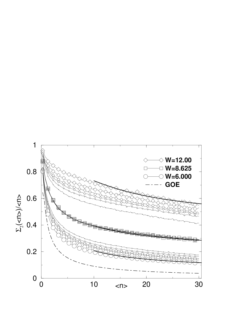
Figure 1: $\Sigma_{2}(\langle n\rangle)/\langle n\rangle$ for coupled planes with $t_{z}=0.1$ and for linear system sizes $N=13,17,21,24,30$ and $40$ denoted by increasing symbol size. The dashed line correspond to the GOE. Note that only every $5$th symbol is shown. The three thick solid lines indicate fits according to Equation (13) of data for $\langle n\rangle>15$.

4.2 FSS with integrated $\Sigma_{2}$ data

In order to perform FSS, we could now use the data of Figure 1 and plot them at each value of $\langle n\rangle$ as a function of disorder. However, such an approach is of limited usefulness since it is apriori unclear how to weigh data from different $\langle n\rangle$ values. Furthermore, the fluctuations in the data lead to rather large error bars in the obtained estimates of $\nu$ and $W_{\rm c}$. Instead, we define the integrated quantity

$$\eta(N,W)=\frac{1}{L_{0}}\int_{0}^{L_{0}}\Sigma_{2}(L)dL$$ (12)

with $L=\langle n\rangle$. This is similar to the FSS analysis of $\Delta_{3}$-statistics Mil00 . The integral is also considered up to $L_{0}=30$ only because the relative error in $\Sigma_{2}$ becomes rather large for larger $L_{0}$ values and hence the calculation is less reliable. It is evident from Figure 2 that $\eta(N,W)$ shows the desired system-size dependence for various values of $W$ exhibiting insulating, critical and metallic behavior for $W$ larger, close to, and smaller than $W_{\rm c}\approx 8.625$.

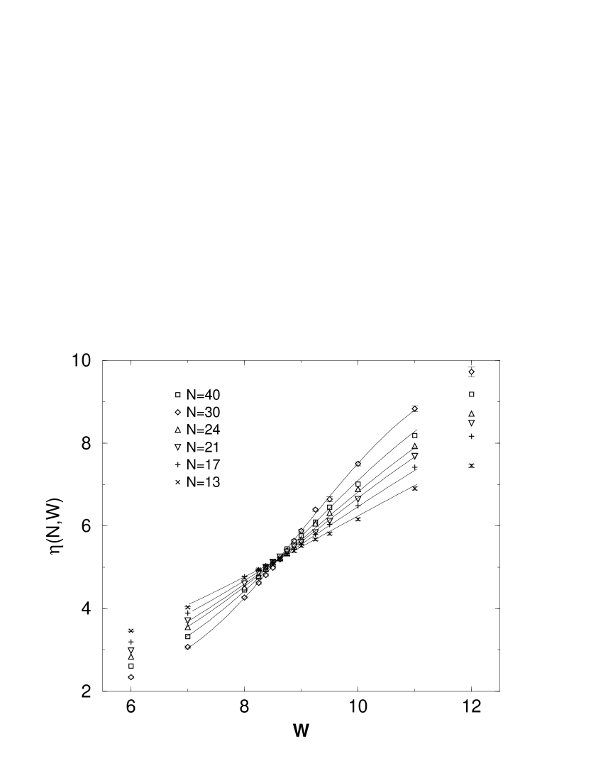
Figure 2: Integrated $\Sigma_{2}$, $\eta(N,W)$, for coupled planes with $t_{z}=0.1$ for linear system sizes shown. The solid lines are fit functions of FSS from Equation (9) with $n_{r}=3$ and $m_{r}=1$.

In order to obtain $\xi$ from finite system-size data we now use the FSS procedure of Section 3. For the non-linear fit, we used the Levenberg-Marquardt method SleO99a . In Figure 3 we show that the data from different system sizes collapse on two branches corresponding to localized and extended behavior. This clearly shows that $\eta$ exhibits one-parameter FSS. We then compute the critical exponent $\nu$ and the critical disorder $W_{\rm c}$ for various parameters. The results are tabulated in Table 1. The average values are $\nu\approx 1.43\pm 0.13$ and $W_{\rm c}\approx 8.62\pm 0.04$, respectively. Here and in the following, the error intervals are standard errors, i.e., denoting one standard deviation.

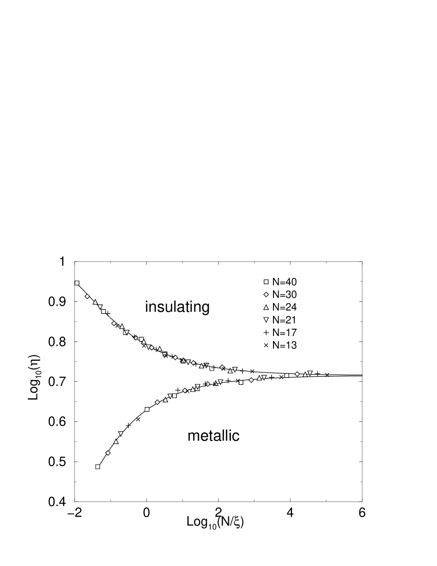
Figure 3: The one-parameter scaling dependence of $\eta$ on $\xi$ for different system sizes $N$ and disorders $W\in[6,12]$.

Table 1: Parameters for FSS of $\eta$ and the resulting estimates for $\nu$ and $W_{\rm c}$. The numbers in the $3$rd and $4$th column denote orders $n_{\rm r}$ and $m_{\rm r}$ used in the expansions (10) and (11), respectively, for which the best fits have been obtained. Q is the goodness-of-fit defined as usual by the $\chi^{2}$ quality of fit PreTVF92 and quoted errors correspond to one standard deviation.

$W$	$N$	$n_{\rm r}$	$m_{\rm r}$	$Q$	$W_{\rm c}$	$\nu$
$7\cdots 11.0$	$13\cdots 40$	$3$	$1$	$0.01$	$8.59(3)$	$1.38(3)$
$7\cdots 11.0$	$13\cdots 40$	$1$	$3$	$0.09$	$8.56(4)$	$1.57(4)$
$8\cdots 9.25$	$13\cdots 40$	$3$	$1$	$0.70$	$8.62(3)$	$1.35(12)$
$8\cdots 9.25$	$13\cdots 40$	$1$	$3$	$0.54$	$8.61(3)$	$1.33(9)$
$8\cdots 9.25$	$13\cdots 40$	$3$	$2$	$0.75$	$8.64(4)$	$1.35(13)$
$8\cdots 9.25$	$13\cdots 40$	$2$	$3$	$0.79$	$8.64(2)$	$1.27(10)$
$8\cdots 9.25$	$24\cdots 40$	$3$	$3$	$0.76$	$8.64(3)$	$1.29(15)$
$7\cdots 11.0$	$24\cdots 40$	$3$	$1$	$0.14$	$8.63(6)$	$1.48(13)$
$7\cdots 11.0$	$24\cdots 40$	$1$	$3$	$0.02$	$8.61(8)$	$1.80(18)$
$8\cdots 9.25$	$24\cdots 40$	$3$	$1$	$0.72$	$8.66(6)$	$1.50(26)$
$8\cdots 9.25$	$24\cdots 40$	$1$	$3$	$0.67$	$8.64(5)$	$1.47(22)$
$7\cdots 11.0$	$13\cdots 40$	$3$	$3$	$0.03$	$8.60(3)$	$1.34(7)$
average:					$8.62(4)$	$1.43(13)$

4.3 FSS with $\chi$

We now turn our attention to computing $\chi$. First we note that $\Sigma_{2}(L)/L$ ($L\equiv\langle n\rangle$) as plotted in Figure 1 is already a crude approximation of $\chi$. Since there is a systematic size dependence, this already indicates that $\chi$ should obey FSS. In order to proceed more accurately, we now fit the ${\Sigma_{2}(L)}/{L}$ data with an ansatz function containing irrelevant scaling exponents $y_{k}$, i.e.

$${\frac{\Sigma_{2}(N,W,L)}{L}}\approx\chi+\sum_{k=1}^{m}a_{k}(N,W)L^{-y_{k}}$$ (13)

up to order $m$. Thus in the limit $L\rightarrow\infty$, the constant term will be equal to the desired value of the level compressibility $\chi$. The data used in the fits range from $L=0$ up to $L\approx 140$. Data for larger $L$ values ($\approx 250$) was ignored due to reduced statistical accuracy. In Figure 1, we show some typical fits for large system sizes.

We next perform FSS of $\chi$ as explained above. However, a non-linear-fit procedure of (increasingly fluctuating) large $L$-data with exponents as fitting parameters is inherently unstable. Thus it is numerically much better to fit with fixed exponents. Using such a fit with $W=7,\ldots,11$, $N=24,\ldots,50$ for $m=1$, we find that $\chi$ ranges from $0.275$ to $0.292$ with $y_{1}$ varying from $0.95$ to $1.3$, respectively. Various other combinations for values of $y_{1}=0.95,\ldots,1.3$ and $y_{2}=1.5,\ldots,2.5$ result in the averaged FSS estimate $\chi_{\rm c}=0.28\pm 0.03$. Other values outside these ranges do not fit ${{\Sigma_{2}(N,W,L)}/{L}}$ and larger values for $m$ do not enhance the quality of the FSS.

As shown, e.g. for $y_{1}=1$ and $y_{2}=2$ in Figure 4, $\chi$ data for different system sizes and $W$ collapse onto a single scaling curve with two branches. From this and further data for different ranges of $W$ and $N$, we can roughly estimate $\chi_{\rm c}$ at the MIT to be $0.28\pm 0.06$ as shown in Table 2. This value is in good agreement with previously obtained estimates ZhaK95b ; Met98 ; Can96 . We also note that Equation (3) with $\kappa=1/2\chi_{\rm c}\approx 1.8$ fits the large-$s$ tails of $P(s)$ at the MIT reasonably well.

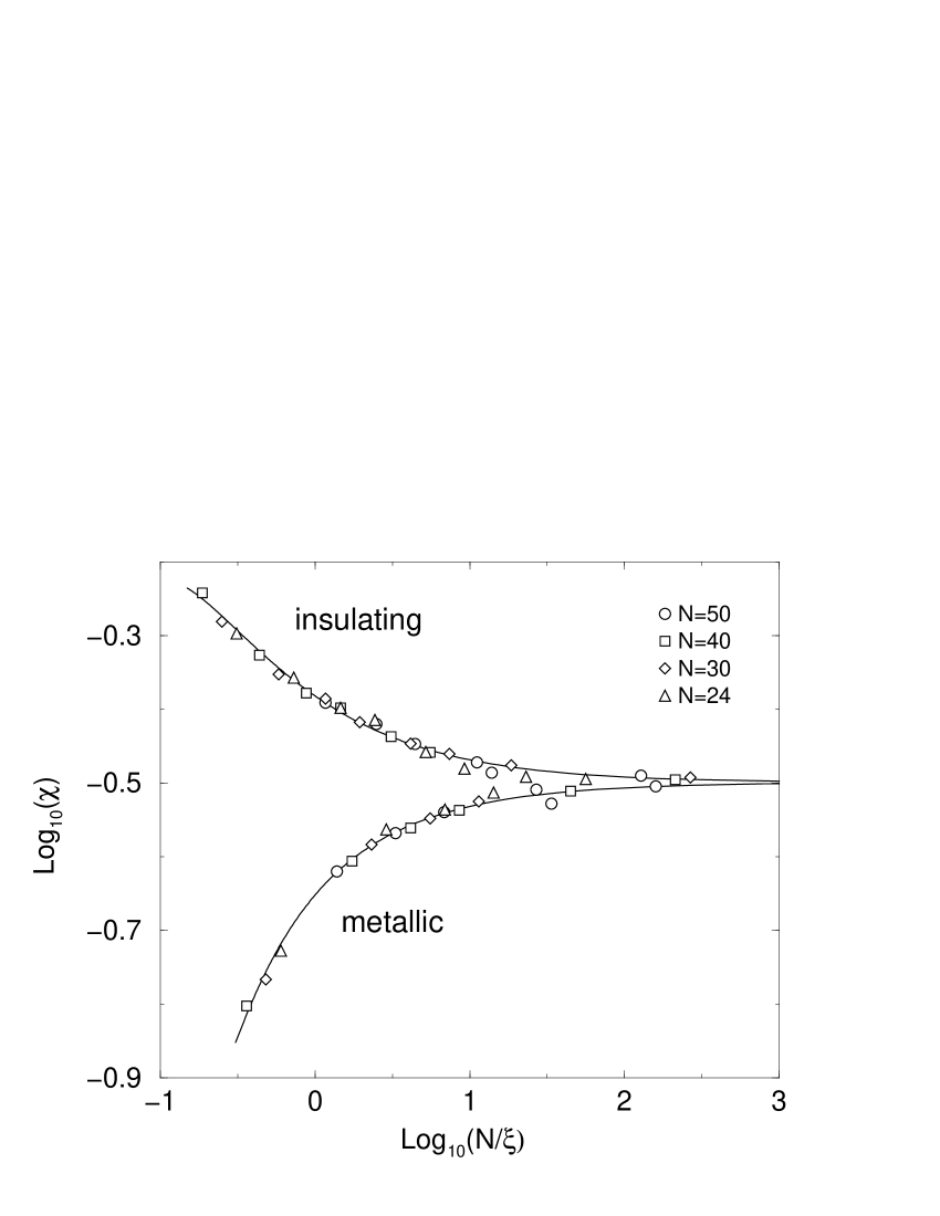
Figure 4: The one-parameter scaling dependence of $\chi$, obtained from Equation (13) for, e.g., $y_{1}=1$ and $y_{2}=2$, on $\xi$ for disorders $W\in[7,11]$, system sizes $24$, $30$, $40$, and $50$, with $n_{\rm r}=3$, $m_{\rm r}=1$. The dashed line indicates the value $\chi_{\rm c}=0.27(1)$ at the MIT obtained from this fit.

Unfortunately, the fit in $L^{-y_{k}}$ is not good enough to reproduce the values for $\nu$ and $W_{\rm c}$ with the desired high accuracy as shown, e.g., in Table 2. This is because the data for large $L$ fluctuate much more strongly than at small $L$ due to the reduced statistics of such extremely large spacings. E.g., even for a system of size $50^{3}$, we have only 250 spacings with $L=250$ available when taking only the central half of the spectrum into consideration to avoid distortions from the localized states in the band tails. Furthermore, the usual unfolding procedures rely on local spectral interpolations and may no longer work for such large spacings. In fact, using an unfolding suitable for small $L$ statistics, we could erroneously reduce the estimated value of $\chi_{\rm c}$ to $\approx 0.25$.

4.4 FSS with $\chi$ from truncated data.

In order to suppress the problems with large-$L$ fluctuations, we have truncated the $\Sigma_{2}/L$ data at $L=30$ and performed the FSS procedure as before with Equation (13) using fixed $y_{1}=1$ and $y_{2}=2$. As shown in Figure 5, the $\chi$ data for different system sizes and different $W$ values collapse again onto a single scaling curve with two branches. Due to the truncation, the estimated values $\chi_{+}$ can only serve as upper limits to the true value $\chi_{\rm c}$ at the MIT. But the resulting values for $\nu$ and $W_{\rm c}$ are of much better accuracy and are shown in Table 2. For the average critical exponent we obtain $\nu\approx 1.44\pm 0.13$ and for the average critical disorder $W_{\rm c}\approx 8.66\pm 0.04$.

Figure 5: The one-parameter scaling dependence of $\chi_{+}$, obtained from Equation (13) for $y_{1}=1$ and $y_{2}=2$ fitted up to $L=30$, on $\xi$ for disorders $W\in[7,11]$, system sizes $24$, $30$, $40$, and $50$, with $n_{\rm r}=3$, $m_{\rm r}=1$.

4.5 FSS with a polynomial fit

In order to proceed more accurately with the determination of $\nu$ and $W_{\rm c}$, we now fit $\Sigma_{2}(L)$ data for small $L$ with a polynomial in $L$, i.e.,

$$\frac{\Sigma_{2}(N,W,L)}{L}\approx\chi_{\rm p}+\sum_{k=1}^{m}b_{k}(N,W)L^{k}$$ (14)

up to order $m$. We then identify a rough estimate of the level compressibility with the linear expansion coefficient $\chi_{\rm p}$. This implies a systematic shift of $\chi$ and the value of $\chi_{\rm p}$ at the MIT will also be shifted towards a larger value when compared to $\chi_{\rm c}$. However, $\nu$ and $W_{\rm c}$ can be determined with increased precision: the quality of the fit, cp. Figure 6, is very good and certainly better than in the two previous cases. As a check to the numerical reliability of this method, we vary the value of $L$ included in the fit function (14) by fitting the $\Sigma_{2}/L$ data for various ranges of $L=10,15,20,25$ and $30$. We find that there is only a negligible change in the obtained values of $\nu$ and $W_{\rm c}$.

Figure 6: $\chi_{\rm p}(N,W)$ obtained by fitting the $\Sigma_{2}$ data with $m=3$ in Equation (14). System-size dependence is clearly seen. The solid lines are fit functions from FSS of Equation (9) with $n_{r}=3$ and $m_{r}=1$.

After FSS, $\chi_{\rm p}$ data for all system sizes and all $W$ collapse onto two curves as shown in Figure 7. Results for $\nu$ and $W_{\rm c}$ for various FSS functions and different $m$ are shown in Table 3. For the average critical exponent we obtain $\nu\approx 1.47\pm 0.10$ and for the average critical disorder $W_{\rm c}\approx 8.56\pm 0.05$.

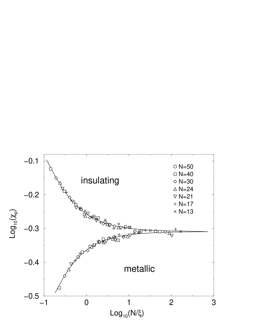
Figure 7: The one-parameter scaling dependence of $\chi_{\rm p}$ on $\xi$ for different system sizes $N$ and disorders $W\in[6,12]$.

The values of $\nu$ calculated from the $\eta$- and the three $\chi$-based approaches are compatible with each other and are also comparable to values from other methods Sch99a ; SleMO01 , for instance the transfer-matrix method which gives $\nu\approx 1.62\pm 0.07$ MilRSU00 . We can therefore claim that both $\chi$ and $\eta$ are good FSS parameters to characterize the MIT. Nevertheless, a simple fitting procedure in the large $L$ limit, although in principle correct, will encounter many numerical problems.

5 Conclusion

States at the 3D MIT are multifractal entities SchG91 ; WEH2000 . This implies that, while not being extended, their spatial structure nevertheless results in a long-ranged, power-law overlap of electronic densities in energy ChaKL96 ; KraM97 , i.e.,

$$\langle|\Psi_{i}|^{2}|\Psi_{k}|^{2}\rangle\propto|E_{i}-E_{k}|^{-(1-D_{2}/d)}$$ (15)

where $D_{2}$ is the correlation dimension MilRS97 and the connection $\chi_{\rm c}=(d-D_{2})/2d$ has been conjectured ChaKL96 . In order to describe generic features of such multifractal states, various critical random matrix models have been suggested and studied MosNS94 ; KraM97 ; AltL97 ; Mir96 ; MutCIN93 , albeit mostly for the unitary class of models. Using the above relation of $D_{2}$ (see Refs. MilRS97 ; Mil00 for numerical estimates at the MIT in anisotropic 3D AMs) with $\chi_{\rm c}$, we find that the computed value $\chi_{\rm c}=0.28\pm 0.06$ is compatible with $D_{2}\approx 1.3\pm 0.1$, which can be calculated easily from the $f(\alpha)$ spectra published in Refs. MilRS97 ; Mil00 ; SchMRE99 . On the other hand, it has been shown that in the limit of “strong multifractality”, the above connection between $\chi_{c}$ and $D_{2}$ no longer holds EveM00 . Previous estimates of $D(2)$ in the isotropic 3D AM range from $1.4$–$1.7$ BraHS96 ; BraMP98 ; ChaKL96 ; KawKO99 ; OhtK96 ; ZhoZSP00 . Certainly, our multifractal Mil00 ; MilRS97 is not an infinitely sparse multifractal wave ($D(2)=0)$) as sometimes expected for the critical ensembles KraM97 .

In summary, our results show that $\chi$ (and $\eta$) can indeed be used to compute, with the help of FSS, estimates of $\chi_{\rm c}$, $W_{\rm c}$ and $\nu$ which are in good agreement with transfer-matrix and other spectral analysis. We are confident that the remaining small difference in values can be further shrunk when larger system sizes become available for the spectral statistics.

Appendix A Another FSS procedure

In a recent communication to the cond-mat archives Sus01 , the FSS method used in the present paper has been criticized and the results obtained by various groups SleO99a ; SleO99b ; OhtSK99 ; MilRSU00 ; MilRS99a ; MilRS01 ; CaiRS99 ; BisCRS00 ; ZhaK98 ; ZhaK97 for the critical exponent $\nu$ of the localization length at the MIT in the 3D AM have been questioned. These claims are based on the observation that there still is some disagreement between analytical, numerical and experimental results for the critical exponent KraM93 . Ref. Sus01 proposes yet another procedure to deal with corrections to scaling. Furthermore, it is hinted that the numerical data support $\nu\approx 1$, whereas the present manuscript and recent numerical papers find $\nu\approx 1.5\pm 0.2$ SleO99a ; SleO99b ; OhtSK99 .

We have tested the method proposed by Ref. Sus01 first with transfer-matrix data MilRSU00 ; CaiRS99 ; BisCRS00 with $\varepsilon\leq 0.1\%$; we find $\nu=1.75\pm 0.17$ for the anisotropic and $1.55\pm 0.04$ for the random-hopping AM. The FSS of section 3 gives $\nu=1.61\pm 0.07$ MilRSU00 and $\nu=1.54\pm 0.03$ CaiRS99 ; BisCRS00 , respectively, for the same set of data. Note that the first value ($1.75$) is so high because systematic shifts of $W_{\rm c}$ due to an irrelevant scaling variable are not taken into account in Sus01 . Using for a second test the energy-level-statistics data of the present manuscript with $\varepsilon\approx 1\%$, we find $\nu=1.51\pm 0.25$. Last, for artificially generated data with precisely known $W_{c}=16.5$ and varying $\nu\in[0.5,2.0]$ the results of the method of Ref. Sus01 are comparable to the results of the Kramer/MacKinnon FSS MacK83 and slightly less reliable than the present FSS as shown in Figure 8.

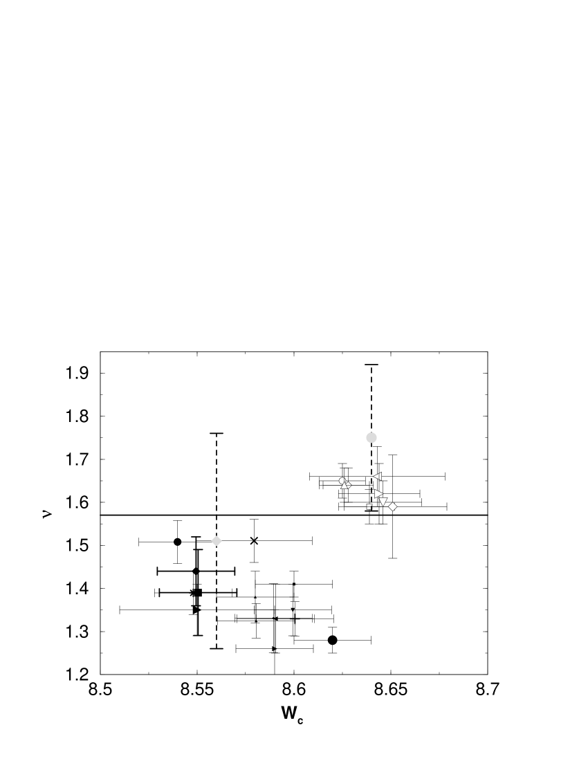
Figure 8: Results for $W_{c}$ and $\nu$, for the anisotropic AM MilRSU00 ; MilRS99a using FSS of Ref. SleO99a for transfer-matrix data (open symbols) and level-statistics data (filled symbols) for various fit functions. The error bars show the $95\%$ confidence intervals. The accuracy of the localization length data obtained from the transfer matrix method is an order of magnitude higher than that of the energy-level-statistics data. The system sizes of transfer-matrix data are larger than for level-statistics data, giving systematically larger $\nu$ values for the former. The goodness of a fit is reflected in the size of the symbol. The $2$ thick error bars mark high quality fits of level-statistics data for large system sizes. The gray $\circ$ and $\Box$ and the corresponding dashed error bars represent the result of the fit procedure of Ref. Sus01 applied to transfer-matrix data and level-statistics data for the anisotropic AM, respectively. The solid line marks the result of Ref. SleO99a .

We conclude that the method proposed in Ref. Sus01 also yields $\nu\approx 1.58$ and not $\nu\approx 1$ for the MIT of the AM.

Table 2: Parameters for FSS of $\chi$ as in (13) with $y_{1}=1$, $y_{2}=2$ and the resulting estimates for $\chi_{\rm c}$, $\nu$ and $W_{\rm c}$. The numbers in the $3$rd and $4$th column denote orders $n_{\rm r}$ and $m_{\rm r}$ used in the expansions (10) and (11), respectively, for which the best fits have been obtained. The $5$th column is for fits based on $\Sigma_{2}$ data up to $L=140$, the $6-8$th columns are for fits up to $L=30$ only. The goodness-of-fit $Q$ PreTVF92 is less than $0.1$ in all cases.

				$L_{\rm max}=140$	$L_{\rm max}=30$
$W$	$N$	$n_{\rm r}$	$m_{\rm r}$	$\chi$	$\chi_{+}$	$W_{\rm c}$	$\nu$
$7\cdots 11.0$	$13\cdots 50$	$3$	$1$	$0.27(9)$	$0.31(5)$	$8.69(3)$	$1.44(7)$
$7\cdots 11.0$	$13\cdots 50$	$1$	$3$	$0.16(3)$	$0.31(3)$	$8.69(3)$	$1.58(8)$
$8\cdots 9.25$	$13\cdots 50$	$3$	$1$	$0.26(12)$	$0.30(5)$	$8.69(4)$	$1.38(16)$
$8\cdots 9.25$	$13\cdots 50$	$1$	$3$	$--$	$0.31(5)$	$8.68(3)$	$1.44(14)$
$8\cdots 9.25$	$13\cdots 50$	$3$	$2$	$0.31(1)$	$0.33(1)$	$8.70(4)$	$1.35(15)$
$8\cdots 9.25$	$13\cdots 50$	$2$	$3$	$0.37(2)$	$0.37(6)$	$8.70(3)$	$1.32(16)$
$8\cdots 9.25$	$24\cdots 50$	$3$	$3$	$0.27(1)$	$0.32(1)$	$8.60(3)$	$1.11(16)$
$7\cdots 11.0$	$24\cdots 50$	$3$	$1$	$0.27(1)$	$0.32(1)$	$8.60(4)$	$1.58(12)$
$7\cdots 11.0$	$24\cdots 50$	$1$	$3$	$0.26(2)$	$0.32(1)$	$8.60(5)$	$1.78(10)$
$8\cdots 9.25$	$24\cdots 50$	$3$	$1$	$0.19(13)$	$0.32(1)$	$8.61(4)$	$1.42(17)$
$8\cdots 9.25$	$24\cdots 50$	$1$	$3$	$0.36(18)$	$0.32(2)$	$8.60(4)$	$1.45(15)$
$7\cdots 11.0$	$13\cdots 50$	$3$	$3$	$0.31(1)$	$0.33(1)$	$8.70(3)$	$1.38(10)$
average:				$0.28(6)$	$0.32(3)$	$8.66(4)$	$1.44(13)$

Table 3: Values of the critical disorder strength $W_{\rm c}$ and the critical exponent $\nu$ values computed from Equation (14) with various $m$ values. The numbers in the $4$th and $5$th column denote orders $n_{\rm r}$ and $m_{\rm r}$ used in the expansions (10) and (11), respectively for which the best fits have been obtained. The goodness-of-fit $Q$ PreTVF92 is larger than $0.99$ in all cases.

$m$	$W$	$N$	$n_{\rm r}$	$m_{\rm r}$	$W_{\rm c}$	$\nu$
2	$7\cdots 11.0$	$13\cdots 50$	$3$	$1$	$8.65(2)$	$1.36(3)$
2	$7\cdots 11.0$	$13\cdots 50$	$1$	$3$	$8.63(2)$	$1.52(4)$
2	$8\cdots 9.25$	$24\cdots 50$	$3$	$1$	$8.57(3)$	$1.43(6)$
2	$8\cdots 9.25$	$24\cdots 50$	$1$	$3$	$8.53(3)$	$1.65(7)$
average:					$8.60(3)$	$1.49(5)$
3	$7\cdots 11.0$	$13\cdots 50$	$3$	$1$	$8.67(2)$	$1.29(3)$
3	$7\cdots 11.0$	$13\cdots 50$	$1$	$3$	$8.61(1)$	$1.42(3)$
3	$8\cdots 9.25$	$24\cdots 50$	$3$	$1$	$8.55(4)$	$1.45(8)$
3	$8\cdots 9.25$	$24\cdots 50$	$1$	$3$	$8.53(4)$	$1.51(8)$
average:					$8.59(3)$	$1.42(6)$
4	$7\cdots 11.0$	$13\cdots 50$	$3$	$1$	$8.54(4)$	$1.32(9)$
4	$7\cdots 11.0$	$13\cdots 50$	$1$	$3$	$8.51(4)$	$1.40(9)$
4	$8\cdots 9.25$	$24\cdots 50$	$3$	$1$	$8.45(10)$	$1.56(26)$
4	$8\cdots 9.25$	$24\cdots 50$	$1$	$3$	$8.42(11)$	$1.68(28)$
average:					$8.48(7)$	$1.49(18)$
total average:					$8.56(5)$	$1.47(10)$

References

- (1) B. Kramer and A. MacKinnon, Rep. Prog. Phys. 56, 1469 (1993).
- (2) P. A. Lee and T. V. Ramakrishnan, Rev. Mod. Phys. 57, 287 (1985).
- (3) P. W. Anderson, Phys. Rev. 109, 1492 (1958).
- (4) Localization 1999: Disorder and Interaction in Transport Phenomena, edited by M. Schreiber, Ann. Phys. (Leipzig) Vol. 8, pp. 531–798, (Wiley-VCH, Berlin, 1999).
- (5) D. Vollhardt and P. Wölfle, Phys. Rev. Lett. 48, 699 (1982).
- (6) D. Vollhardt and P. Wölfle, in Electronic Phase Transitions, edited by W. Hanke and Y. V. Kopaev (North-Holland, Amsterdam, 1992), p. 1.
- (7) J.-L. Pichard and G. Sarma, J. Phys. C 14, L127 (1981).
- (8) J.-L. Pichard and G. Sarma, J. Phys. C 14, L617 (1981).
- (9) A. MacKinnon and B. Kramer, Phys. Rev. Lett. 47, 1546 (1981).
- (10) A. MacKinnon and B. Kramer, Z. Phys. B 53, 1 (1983).
- (11) K. Binder, Rep. Prog. Phys. 60, 487 (1997).
- (12) B. Kramer and M. Schreiber, in Computational Physics, edited by K. H. Hoffmann and M. Schreiber (Springer, Berlin, 1996), pp. 166–188.
- (13) M. Schreiber, B. Kramer, and A. MacKinnon, Physica Scripta T25, 67 (1989).
- (14) B. Kramer, A. Broderix, A. MacKinnon, and M. Schreiber, Physica A 167, 163 (1990).
- (15) E. Hofstetter and M. Schreiber, Europhys. Lett. 21, 933 (1993).
- (16) A. MacKinnon, J. Phys.: Condens. Matter 6, 2511 (1994).
- (17) K. Slevin and T. Ohtsuki, Phys. Rev. Lett. 82, 382 (1999), ArXiv: cond-mat/9812065.
- (18) K. Slevin and T. Ohtsuki, Phys. Rev. Lett. 82, 669 (1999).
- (19) T. Ohtsuki, K. Slevin, and T. Kawarabayashi, Ann. Phys. (Leipzig) 8, 655 (1999), ArXiv: cond-mat/9911213.
- (20) F. Milde, R. A. Römer, M. Schreiber, and V. Uski, Eur. Phys. J. B 15, 685 (2000), ArXiv: cond-mat/9911029.
- (21) F. Milde, R. A. Römer, and M. Schreiber, Phys. Rev. B 61, 6028 (2000), ArXiv: cond-mat/9909210.
- (22) F. Milde, R. A. Römer, and M. Schreiber, in Proc. 25th Int. Conf. Phys. Semicond., edited by N. Miura and T. Ando (Springer, Tokio, 2001), pp. 148–149, ArXiv: cond-mat/0009469.
- (23) P. Cain, R. A. Römer, and M. Schreiber, Ann. Phys. (Leipzig) 8, SI33 (1999), ArXiv: cond-mat/9908255.
- (24) P. Biswas, P. Cain, R. A. Römer, and M. Schreiber, phys. stat. sol. (b) 218, 205 (2000), ArXiv: cond-mat/0001315.
- (25) I. K. Zharekeshev and B. Kramer, Ann. Phys. (Leipzig) 7, 442 (1998), ArXiv: cond-mat/9810286.
- (26) I. K. Zharekeshev and B. Kramer, Phys. Rev. Lett. 79, 717 (1997), ArXiv: cond-mat/9706255.
- (27) P. Cain, M. L. Ndawana, R. A. Römer, and M. Schreiber, (2001), ArXiv: cond-mat/0106005.
- (28) H. Stupp, M. Hornung, M. Lakner, O. Madel, and H. v. Löhneysen, Phys. Rev. Lett. 71, 2634 (1993).
- (29) S. Waffenschmidt, C. Pfleiderer, and H. v. Löhneysen, Phys. Rev. Lett. 83, 3005 (1999), ArXiv: cond-mat/9905297.
- (30) S. Bogdanovich, M. P. Sarachik, and R. N. Bhatt, Phys. Rev. Lett. 82, 137 (1999).
- (31) S. Bogdanovich, M. P. Sarachik, and R. N. Bhatt, Ann. Phys. (Leipzig) 8, 639 (1999).
- (32) K. M. Itoh, M. Watanabe, Y. Ootuka, and E. E. Haller, Ann. Phys. (Leipzig) 8, 631 (1999).
- (33) T. F. Rosenbaum, G. A. Thomas, and M. A. Paalanen, Phys. Rev. Lett. 72, 2121 (1994).
- (34) H. Stupp, M. Hornung, M. Lakner, O. Madel, and H. v. Löhneysen, Phys. Rev. Lett. 72, 2122 (1994).
- (35) T. G. Castner, Phys. Rev. Lett. 87, 129701 (2001).
- (36) E. Abrahams, P. W. Anderson, D. C. Licciardello, and T. V. Ramakrishnan, Phys. Rev. Lett. 42, 673 (1979).
- (37) B. L. Altshuler and B. I. Shklovskii, Zh. Eksp. Teor. Fiz. 91, 220 (1986), [Sov. Phys. JETP 64, 127 (1986)].
- (38) V. E. Kravtsov, I. V. Lerner, B. L. Altshuler, and A. G. Aronov, Phys. Rev. Lett. 72, 888 (1994).
- (39) E. P. Wigner, Ann. Math. 62, 548 (1955).
- (40) E. P. Wigner, Ann. Math. 65, 203 (1957).
- (41) F. J. Dyson, J. Math. Phys. 3, 140 (1962).
- (42) M. L. Mehta, Random Matrices (Academic Press, Boston, 1990).
- (43) K. B. Efetov, Adv. Phys. 32, 53 (1983).
- (44) B. I. Shklovskii, B. Shapiro, B. R. Sears, P. Lambrianides, and H. B. Shore, Phys. Rev. B 47, 11487 (1993).
- (45) E. Hofstetter and M. Schreiber, Phys. Rev. B 49, 14726 (1994), ArXiv: cond-mat/9402093.
- (46) V. E. Kravtsov and K. A. Muttalib, Phys. Rev. Lett. 79, 1913 (1997), ArXiv: cond-mat/9703167; V. E. Kravtsov, in Proceedings of the Correlated Fermions and Transport in Mesoscopic Systems, Moriond Conference, Les Arcs (1996), ArXiv: cond-mat/9603166.
- (47) B. L. Altshuler, I. K. Zharekeshev, S. A. Kotochigova, and B. I. Shklovskii, Zh. Eksp. Teor. Fiz. 94, 343 (1988), [Sov. Phys. JETP 67, 625 (1988)].
- (48) M. Metzler, J. Phys. Soc. Japan 67, 4006 (1998), ArXiv: cond-mat/9809340; M. Metzler and I. Varga, J. Phys. Soc. Japan 67, 1856 (1998); M. Metzler, J. Phys. Soc. Japan 68, 144 (1999).
- (49) E. Bogomolny, U. Gerland and C. Schmit, Eur. Phys. J. B 19, 121 (2001).
- (50) I. K. Zharekeshev and B. Kramer, in Quantum Dynamics in Submicron Structures, edited by H. A. Cerdeira, B. Kramer, and G. Schön, NATO ASI Ser. E 291, p. 93 (Kluwer, Dordrecht, 1994), ArXiv: cond-mat/0112171.
- (51) A. D. Mirlin, Phys. Rep. 326, 259 (2000).
- (52) A. G. Aronov and A. Mirlin, Phys. Rev. B 51, 6131 (1995).
- (53) V. E. Kravtsov and I. V. Lerner, Phys. Rev. Lett. 74, 2563 (1995).
- (54) A. G. Aronov, V. E. Kravtsov, and I. V. Lerner, Pis’ma Zh. Eksp. Teor. Fiz. 59, 50 (1994), [Sov. Phys. JETP 59, 39 (1994)].
- (55) D. Braun, G. Montambaux, and M. Pascaud, Phys. Rev. Lett. 81, 1062 (1998), ArXiv: cond-mat/9712256.
- (56) I. M. Suslov, (2001), ArXiv: cond-mat/0105325.
- (57) K. Slevin and T. Ohtsuki, Phys. Rev. Lett. 78, 4083 (1997), ArXiv: cond-mat/9704192.
- (58) I. Zambetaki, Q. Li, E. N. Economou, and C. M. Soukoulis, Phys. Rev. Lett. 76, 3614 (1996), cond-mat/9704107; I. Zambetaki, Q. Li, E. N. Economou, and C. M. Soukoulis, Phys. Rev. Lett. 77, 3266 (1996); I. Zambetaki, Q. Li, E. N. Economou, and C. M. Soukoulis, Phys. Rev. B 56, 12223 (1996).
- (59) F. Milde, Dissertation, Technische Universität Chemnitz (2000).
- (60) J. Cullum and R. A. Willoughby, Lanczos Algorithms for Large Symmetric Eigenvalue Computations, Volume 1: Theory and Volume 2: Programs (Birkhäuser, Boston, 1985), http://www.netlib.org/lanczos/.
- (61) H. E. Stanley, Introduction to Phase Transitions and Critical Phenomena (Oxford University Press, New York, 1987)
- (62) F. Siringo and G. Piccitto, J. Phys. A: Math. Gen. 31, 5981 (1998), ArXiv: cond-mat/9706127.
- (63) F. Milde, R. A. Römer, and M. Schreiber, Phys. Rev. B 55, 9463 (1997).
- (64) W. H. Press, S. A. Teukolsky, W. T. Vetterling, B. P. Flannery Numerical Recipes in Fortran 77: The Art of Scientific Computing (Cambridge University Press, Boston, 1992).
- (65) I. K. Zharekeshev and B. Kramer, Jpn. J. Appl. Phys., 34, 4361 (1995), ArXiv: cond-mat/9506114.
- (66) C. M. Canali, Phys. Rev. B 53, 3713 (1996).
- (67) K. Slevin, P. Markoš and T. Ohtsuki, Phys. Rev. Lett. 86, 3594 (2001).
- (68) M. Schreiber and H. Grussbach, Phys. Rev. Lett. 67, 607 (1991).
- (69) K. H. Hoffmann, M. Schreiber (Eds.), Computational Statistical Physics: From Billiards to Monte Carlo (Springer-Verlag, Berlin, 2001)
- (70) J. Chalker, V. Kravtsov, and I. Lerner, Pis’ma Zh. Eksp. Teor. Fiz. 64, 355 (1996), [Sov. Phys. JETP Lett. 64, 386 (1996)].
- (71) M. Moshe, H. Neuberger, and B. Shapiro, Phys. Rev. Lett. 73, 1497 (1994).
- (72) B. L. Altshuler and L. S. Levitov, (1997), ArXiv: cond-mat/9704122.
- (73) A. D. Mirlin, Phys. Rev. B 53, 1186 (1996).
- (74) K. A. Muttalib, Y. Chen and V. N. Nicopoulos, Phys. Rev. Lett. 71, 471 (1993).
- (75) M. Schreiber, F. Milde, R. A. Römer, U. Elsner, and V. Mehrmann, Comp. Phys. Comm. 121–122, 517 (1999).
- (76) F. Evers and A. D. Mirlin, Phys. Rev. Lett. 84, 3690 (2000).
- (77) T. Brandes, B. Huckestein, and L. Schweitzer, Ann. Phys. (Leipzig) 5, 633 (1996).
- (78) T. Kawarabayashi, B. Kramer, and T. Ohtsuki, Ann. Phys. (Leipzig) 8, 487 (1999), ArXiv: cond-mat/9907319.
- (79) T. Ohtsuki and T. Kawarabayashi, J. Phys. Soc. Japan 66, 314 (1996).
- (80) J. Zhong, Z. Zhang, M. Schreiber, E. W. Plummer, and Q. Niu, (2000), ArXiv: cond-mat/0011118.