Field Dependence of Electronic Specific Heat in Two-Band Superconductors

Much attention has been focused on the recently discovered MgB₂ because of its relatively high superconducting transition temperature $T_{\rm c}\sim$ 39K and simple crystalline structure.${}^{\hbox{\immediate{\bf{?}})}}$ General consensus obtained so far is that the electron-phonon interaction is mainly responsible for the pairing mechanism in this system because the large isotope effect is observed.${}^{\hbox{\immediate{\bf{?}},\penalty 1000\hskip 0.91003pt plus 0.70004pt minus 0.70004pt{\bf{?}})}}$ There is, however, little consensus as to the microscopic description for the record high $T_{\rm c}$ due to the electron-phonon interaction.

Apart from the much debated pairing mechanism, it is rather urgent to determine the precise pairing function or gap function realized in MgB₂. There are several important, but conflicting experimental data concerning the superconducting energy gap $\Delta$, ranging from the strong electron-phonon coupling $2\Delta/k_{\rm B}T_{\rm c}\sim 5$ to extremely weak coupling value $2\Delta/k_{\rm B}T_{\rm c}\sim 2$. These come from the earlier experiments, such as position-dependent tunneling or Raman experiments.${}^{\hbox{\immediate{\bf{?}})}}$ More recent experiments show unequivocally that these two gap values come from a single sample and converge to definite values: the larger $\Delta_{L}$ and the smaller $\Delta_{S}$ whose ratio $\Delta_{S}/\Delta_{L}$ falls around 0.3$\sim$0.4. These experiments include photoemmision ($\Delta_{L}$=5.6meV, $\Delta_{S}$=1.7meV, $\Delta_{S}/\Delta_{L}$=0.30),${}^{\hbox{\immediate{\bf{?}})}}$ the $T$-dependent specific heat analysis ($\Delta_{S}/\Delta_{L}$=0.27)${}^{\hbox{\immediate{\bf{?}},\penalty 1000\hskip 0.91003pt plus 0.70004pt minus 0.70004pt{\bf{?}})}}$ and tunneling experiment ($\Delta_{S}/\Delta_{L}$=0.42).${}^{\hbox{\immediate{\bf{?}})}}$ Through these analyses, they are able to obtain systematic and smooth $T$ evolutions of each gap value. This implies that the two gap structure is an intrinsic property in MgB₂.

According to the band structure calculations,${}^{\hbox{\immediate{\bf{?}},\penalty 1000\hskip 0.91003pt plus 0.70004pt minus 0.70004pt{\bf{?}})}}$ there are two distinctive Fermi surface sheets; one is a two-dimensional cylindrical Fermi surface arising from $\sigma$-orbitals due to $p_{x}$ and $p_{y}$ electrons of B atoms and the other is a Fermi surface coming from $\pi$-orbitals due to $p_{z}$ electrons of B atoms. They are weakly hybridized with electron orbitals of Mg atoms. Since the $\sigma$-orbital is strongly coupled to the in-plane B-atom vibration with E_2g symmetry simply because the hopping integral between the $\sigma$-orbitals is modulated by this bond stretching motion. On the other hand, it is shown by the band calculation${}^{\hbox{\immediate{?})}}$ that the $\pi$-orbital is weakly coupled with this phonon mode. Thus it is quite conceivable that these two Fermi surfaces with different electronic characters have different energy-gap values if this particular in-plane vibrational mode is responsible for the attractive interaction which induces superconductivity in MgB₂.

Here we are going to analyze the field dependence of the $T$-linear electronic specific-heat coefficient $\gamma(H)$ in the superconducting mixed state by investigating the vortex lattice structure in two-band superconductors. It is known that $\gamma(H)$ is a sensitive and useful quantity to reflect the gap structure through the zero-energy excitation spectrum inside and outside the vortex core.${}^{\hbox{\immediate{\bf{?}},\penalty 1000\hskip 0.91003pt plus 0.70004pt minus 0.70004pt{\bf{?}},\penalty 1000\hskip 0.91003pt plus 0.70004pt minus 0.70004pt{\bf{?}},\penalty 1000\hskip 0.91003pt plus 0.70004pt minus 0.70004pt{\bf{?}})}}$ In particular, the exponent $\alpha$ in $\gamma(H)\propto H^{\alpha}$ at low fields reflects the nodal structure of the superconducting gap at the Fermi surface, playing a vital role to identify the gap function.${}^{\hbox{\immediate{\bf{?}})}}$ Several recent specific heat experiments on MgB₂ show a very small exponent${}^{\hbox{\immediate{?},\penalty 1000\hskip 0.91003pt plus 0.70004pt minus 0.70004pt{\bf{?}},\penalty 1000\hskip 0.91003pt plus 0.70004pt minus 0.70004pt{\bf{?}})}}$ $\alpha\sim 0.23$, implying that on increasing $H$ the zero-energy density of states (DOS) in the mixed state quickly recovers its normal state value, compared with those in $d$-wave superconductors${}^{\hbox{\immediate{?},\penalty 1000\hskip 0.91003pt plus 0.70004pt minus 0.70004pt{?},\penalty 1000\hskip 0.91003pt plus 0.70004pt minus 0.70004pt{?},\penalty 1000\hskip 0.91003pt plus 0.70004pt minus 0.70004pt{?})}}$ with $\alpha\sim 0.5$ or clean limit $s$-wave case${}^{\hbox{\immediate{?},\penalty 1000\hskip 0.91003pt plus 0.70004pt minus 0.70004pt{?})}}$ with $\alpha\sim 0.7$. Since there are no definitive reports which claim a line or point node in the superconducting gap in MgB₂, this small exponent remains mystery and requires a proper explanation by microscopic calculations. This is one of our purposes in this paper based on the microscopic theory of Bogoliubov-de Gennes (BdG) framework.${}^{\hbox{\immediate{?},\penalty 1000\hskip 0.91003pt plus 0.70004pt minus 0.70004pt{\bf{?}},\penalty 1000\hskip 0.91003pt plus 0.70004pt minus 0.70004pt{\bf{?}})}}$

We start with a model pairing Hamiltonian for a two-band superconductor described by tight binding form:

$${\hat{H}} = {\hat{H}}_{0}+{\hat{H}}_{pair},$$ (1)

$${\hat{H}}_{0} = \sum_{i,j,\sigma,\gamma}(-\tilde{t}_{ij\gamma}-\mu_{\gamma}\delta_{i,j})a^{\dagger}_{i\sigma\gamma}a_{j\sigma\gamma},$$ (2)

$${\hat{H}}_{pair} = \frac{1}{2}\sum_{i,\sigma,\gamma,\gamma^{\prime}}g_{\gamma\gamma^{\prime}}(a_{i\sigma\gamma}a_{i-\sigma\gamma})^{\dagger}a_{i\sigma\gamma^{\prime}}a_{i-\sigma\gamma^{\prime}}$$ (3)

with the nearest neighbor (NN) hopping integral

$$\tilde{t}_{ij\gamma} = t_{\gamma}{\rm exp}[{\rm i}\frac{\pi}{\phi_{0}}\int^{{\mbox{\boldmath$r$}}_{j}}_{{\mbox{\boldmath$r$}}_{i}}{\mbox{\boldmath$A$}}({\mbox{\boldmath$r$}})\cdot{\rm d}{\mbox{\boldmath$r$}}],$$ (4)

where ${\mbox{\boldmath$A$}}({\mbox{\boldmath$r$}})$ is the vector potential and $\phi_{0}={hc/2e}$ is the unit flux. The two-dimensional square lattice whose lattice constant is unity is assumed. The index $\gamma$ denotes the two bands $\gamma=L$ and $S$. Assuming the singlet pairing, we can derive the BdG equations for $\gamma=L$ and $S$ in a standard way:

$$\sum_{i}\left(\begin{array}[]{@{\,}cc@{\,}}K_{ji\gamma}&\delta_{i,j}\Delta_{i\gamma}\\ \delta_{i,j}\Delta_{i\gamma}^{\dagger}&-K_{ji\gamma}^{\ast}\end{array}\right)\left(\begin{array}[]{@{\,}c@{\,}}u_{\gamma\epsilon}({\mbox{\boldmath$r$}}_{i})\\ v_{\gamma\epsilon}({\mbox{\boldmath$r$}}_{i})\end{array}\right) = E_{\gamma\epsilon}\left(\begin{array}[]{@{\,}c@{\,}}u_{\gamma\epsilon}({\mbox{\boldmath$r$}}_{j})\\ v_{\gamma\epsilon}({\mbox{\boldmath$r$}}_{j})\end{array}\right)$$ (10)

where

$$K_{ij\gamma}=-\tilde{t}_{ij\gamma}-\mu_{\gamma}\delta_{i,j}.$$ (12)

The gap equation is given by

$$\Delta_{i\gamma}=\sum_{\gamma^{\prime}}g_{\gamma\gamma^{\prime}}d_{\gamma^{\prime}}({\mbox{\boldmath$r$}}_{i})$$ (13)

with the order parameter

$$d_{\gamma}({\mbox{\boldmath$r$}}_{i}) = \langle a_{i\downarrow\gamma}a_{i\uparrow\gamma}\rangle$$ (14)

$$= -\sum_{\epsilon}v^{\ast}_{\gamma\epsilon}({\mbox{\boldmath$r$}}_{i})u_{\gamma\epsilon}({\mbox{\boldmath$r$}}_{i})\tanh{E_{\gamma\epsilon}\over 2T}.$$

The local density of states (LDOS) at site $i$ for the $\gamma$ band is calculated by

$$N_{\gamma}({\mbox{\boldmath$r$}}_{i},E)=\sum_{\epsilon}\{|u_{\gamma\epsilon}({\mbox{\boldmath$r$}}_{i})|^{2}\delta(E-E_{\gamma\epsilon})$$

$$+|v_{\gamma\epsilon}({\mbox{\boldmath$r$}}_{i})|^{2}\delta(E+E_{\gamma\epsilon}) \}.$$ (15)

We assume an isotropic $s$-wave pairing for both bands $\gamma=L$ and $S$ characterized by the order parameters (the energy gaps) $d_{L}(\Delta_{L})$ and $d_{S}(\Delta_{S})$. The attractive interactions are chosen as $g_{LL}\neq 0$, $g_{LS}=g_{SL}\neq 0$ and $g_{SS}=0$, namely in eq. (5) the gap $\Delta_{S}$ on the $S$-band is induced by the Cooper pair tunneling via $g_{LS}$. As for the normal state band parameters we take $t_{L}=t_{S}=t(\equiv 1)$ and $\mu_{L}=-1$ and $\mu_{S}=+1$, thus the Fermi surface for $\gamma=L(S)$ is close (open) around the $\Gamma$-point. The DOS for both bands is same at the Fermi level. As two vortices are accommodated in a unit cell of ${N_{\rm a}\times N_{\rm a}}$ atomic sites, the applied magnetic field is given by $H_{N_{\rm a}{\times}N_{\rm a}}\equiv 2\phi_{0}/N_{\rm a}^{2}$. By introducing the quasi-momentum of the magnetic Bloch state we obtain the wave function under the periodic boundary condition for a large number of unit cells (See detailed numerical calculations in ref. 19).

First, we study the case $g_{LL}=2.0$ and $g_{LS}=0.6$, which gives $\Delta_{L}=0.322$ and $\Delta_{S}=0.086$ at zero field. It is designed to adjust the gap ratio for MgB₂($\Delta_{S}/\Delta_{L}=0.27$). If we consider a single band superconductor with the small gap $\Delta=0.086$, the superconductivity vanishes at the following magnetic field discussed below, since $H>H_{{\rm c}2}$. But, in this two band superconductor, the small gap superconductivity survives in the $S$-band because of the cooper pair transfer $g_{LS}$.

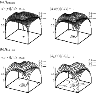
Fig.  1: Spatial profiles of the order parameter $|d_{L}({\mbox{\boldmath$r$}})|$ for the $L$-band and $|d_{S}({\mbox{\boldmath$r$}})|$ for the $S$-band at lower field $H_{30\times 30}$(a) and at higher field $H_{18\times 18}$(b). They are normalized by the zero field values $|d_{L}|_{H=0}(=0.145)$ and $|d_{S}|_{H=0}(=0.055)$, respectively.

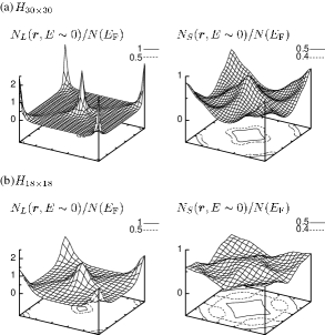
Fig.  2: Zero energy local density of states ${N_{L}({\mbox{\boldmath$r$}},E\sim 0)}$ for the $L$-band and ${N_{S}({\mbox{\boldmath$r$}},E\sim 0)}$ for the $S$-band at lower field $H_{30\times 30}$(a) and at higher field $H_{18\times 18}$(b). They are normalized by $N(E_{\rm F})$, the normal state DOS at the Fermi level.

The spatial profiles of the order parameters $d_{L}({\mbox{\boldmath$r$}})$ and $d_{S}({\mbox{\boldmath$r$}})$ are shown in Fig. 1 where the unit cell of the square vortex lattice is displayed. Vortices are accommodated at the center and four corners. It is seen that the vortex core radius for the $L$-band ($S$-band) is small (large) and the depression of $|d({\mbox{\boldmath$r$}})|$ is apparent along the NN direction, in particular, for the $S$-band. By increasing $H$, $|d({\mbox{\boldmath$r$}})|$ is further suppressed as is seen in Fig. 1 where the core radius is widen. The suppression by $H$ is eminent in the $S$-band.

The corresponding spatial profiles of the LDOS are shown in Fig. 2, where $N_{L}({\mbox{\boldmath$r$}},E\sim 0)$ and $N_{S}({\mbox{\boldmath$r$}},E\sim 0)$ have a peak at the vortex center and the ridges connecting the vortex cores are clearly seen. While the high density of states is concentrated at the vortex core in ${N_{L}({\mbox{\boldmath$r$}},E\sim 0)}$, it rather spreads out in ${N_{S}({\mbox{\boldmath$r$}},E\sim 0)}$. This is because the vortex bound states are highly confined in the $L$-band vortex corresponding to the narrow core radius while in the $S$-band vortex the core states are loosely bounded. The spatial profiles for $N_{L}({\mbox{\boldmath$r$}},E\sim 0)$ and $N_{S}({\mbox{\boldmath$r$}},E\sim 0)$ are resemble to those of the low-field case and the high-field case in the single band superconductor (see Fig. 1 and Fig. 2 in ref. 13). In $N_{S}({\mbox{\boldmath$r$}},E\sim 0)$, the low energy states extending from vortex cores overlap with each other, and the LDOS is suppressed along the line connecting the NN or next NN vortices. With increasing $H$, the effect by the overlap becomes eminent, and the LDOS is reduced to the flat profile $N_{S}({\mbox{\boldmath$r$}},E\sim 0)/N(E_{\rm F})\sim 0.5$ in the $S$-band ($N(E_{\rm F})$ is the total DOS in the normal state at the Fermi level).

The spatial average of ${N_{L}({\mbox{\boldmath$r$}},E\sim 0)}$ and ${N_{S}({\mbox{\boldmath$r$}},E\sim 0)}$ gives rise to the total DOS under a given field, leading to ${\gamma(H)}$ which is defined by

$$\gamma(H)=\gamma_{L}(H)+\gamma_{S}(H)$$ (16)

with

$$\gamma_{L,S}(H)=\langle N_{L,S}({\mbox{\boldmath$r$}},E\sim 0)\rangle_{{\mbox{\boldmath$r$}}:{\rm unit\,cell}}.$$ (17)

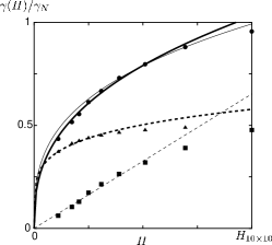
Fig.  3: Field dependence of ${\gamma(H)}$ for ${\Delta_{S}/\Delta_{L}=0.27}$. Points of $\gamma(H)$(circles), $\gamma_{S}(H)$(triangles) and $\gamma_{L}(H)$(squares) are numerical data. The thick line is fitting for lower field data of $\gamma(H)$. The thin line is fitting by ${\gamma(H)\sim\gamma_{N}(H/H_{{\rm c}2})^{\alpha}}$. In the low field the thick(thin) dotted line is fitting for $\gamma_{S}(H)$($\gamma_{L}(H)$).

We have done extensive computations for various $H_{N_{\rm a}\times N_{\rm a}}$cases. In Fig. 3, it is seen that $\gamma(H)$ is described by a power law: $\gamma(H)\propto H^{\alpha}$ with small $\alpha$. If only the low field points are fitted, we obtain ${\alpha=0.38}$(thick line). The fitting by ${\gamma(H)\sim\gamma_{N}(H/H_{{\rm c}2})^{\alpha}}$ under the condition that $\gamma(H)$ is reduced to the normal state value $\gamma_{N}$ gives $\alpha=0.33$(thin line). The small exponents $\alpha$, or the sharp rise of $\gamma(H)$ in small fields, can be attributed to the $S$-band contribution $\gamma_{S}(H)\propto H^{0.20}$, while $\gamma_{L}(H)\propto H^{1.00}$ in the $L$-band. That is, the small $\alpha$ is due to the overlap of the low energy states outside of vortex cores at the $S$-band. Physically it is because the energy gap for the $S$-band is suppressed by a weak field, while the total superconductivity is maintained by the larger energy gap up to $H_{{\rm c}2}$. This intuitively appealing picture is actually confirmed by the present microscopic calculation. This is, however, different from the two independent gaps with different transition temperatures and different $H_{{\rm c}2}$. In such a case, we would have double transitions and $\gamma(H)$ would be a simple addition of two independent curves, which has a kink structure at the lower $H_{{\rm c}2}$. This is not the case for MgB₂.

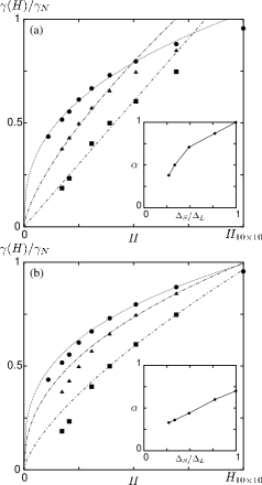
Fig.  4: Field dependence of $\gamma(H)$ for $\Delta_{S}/\Delta_{L}=0.27$(circles), 0.49(triangles) and 0.997(squares). (a)Fitting lines for the low field data. (b)Fitting lines by $\gamma(H)\sim\gamma_{N}(H/H_{\rm c})^{\alpha}$. Points of numerical data are the same in both figures. In the insets, $\Delta_{S}/\Delta_{L}$-dependence of $\alpha$ is shown for each fitting case.

To study the dependence of $\alpha$ on the gap ratio $\Delta_{S}/\Delta_{L}$, we perform the calculation for various pairing parameter sets. In Fig. 4, we show the $\Delta_{S}/\Delta_{L}$-dependence of $\gamma(H)$ behavior. There, we show the results using the two kinds of fitting; the fitting for low field data in Fig. 4(a), and overall fitting by ${\gamma(H)\sim\gamma_{N}(H/H_{{\rm c}2})^{\alpha}}$ in Fig. 4(b), while the numerical data are the same in both figures. In the insets, we show the $\Delta_{S}/\Delta_{L}$-dependence of $\alpha$ in each fitting case. In the limiting case $\Delta_{S}/\Delta_{L}\to 1$, $\alpha$ is reduced to the exponent in the single band case. In Fig. 4(b), it gives $\alpha\sim 0.7$ in accord with the previous quasi-classical calculation.${}^{\hbox{\immediate{?})}}$ In both cases, $\alpha$ monotonically decreases with decreasing $\Delta_{S}/\Delta_{L}$. It should be emphasized that we may identify the gap ratio ${\Delta_{S}/\Delta_{L}}$ uniquely by measuring the electronic specific heat under varying external field, providing a rather unique spectroscopic method for determining the gap ratio. In Fig. 4, for the gap ratio ${\Delta_{S}/\Delta_{L}}\sim 0.3$ observed by the several groups with different methods, we obtain small exponent $\alpha$, as in the specific heat data on MgB₂.

There are several factors which might alter our conclusion on the relation $\alpha$ vs. ${\Delta_{S}/\Delta_{L}}$.

(1) We assume that the DOS in the normal state for each Fermi surface sheet is equal. According to the band calculation by Belashchenko et al.${}^{\hbox{\immediate{\bf{?}})}}$ the ratio of the two DOS is 0.55 ($\pi$-band) : 0.45 ($\sigma$-band). This small difference causes potentially to alter our conclusion, but not in an essential way.

(2) It is assumed that in the minor $S$-band there is no direct attractive interaction $g_{SS}=0$. The gap in the $S$-band is exclusively induced by the Cooper pair tunneling process via $g_{LS}\neq 0$. According to Kortus et al,${}^{\hbox{\immediate{?})}}$ the electron-phonon coupling in the $S$-band due to the bond stretching mode is smaller than that in the $L$-band, but yet non-vanishing. Thus $g_{SS}$ might not completely vanish in MgB₂. We might regard it vanish as a first approximation because our conclusion relies exclusively on the gap ratio ${\Delta_{S}/\Delta_{L}}$. The effect of $g_{SS}\neq 0$ will be studied in the future for more details.

(3) We comment on the small discrepancy of the exponent $\alpha$ between our calculation based on BdG theory and that of the experiment. Since our parameters belong to a rather quantum limit case (the coherent length $\xi$ is an order of the atomic lattice constant), the quasi-classical calculation${}^{\hbox{\immediate{?},\penalty 1000\hskip 0.91003pt plus 0.70004pt minus 0.70004pt{?})}}$ is more appropriate for MgB₂. We believe, however, that the overall relation $\alpha$ vs. ${\Delta_{S}/\Delta_{L}}$ is not greatly altered in that calculation. We will study this case in a future publication.

Haas and Maki${}^{\hbox{\immediate{\bf{?}})}}$ analyze an anisotropic $s$-wave pairing state in connection with MgB₂. Their single band model is designed to describe the anisotropic superconducting properties such as the upper critical field or the penetration depth. According to the recent penetration depth measurement${}^{\hbox{\immediate{\bf{?}})}}$ for single crystals of MgB₂, the anisotropy of the penetration depths for $H\parallel c$ and $H\perp c$ in the hexagonal crystal is almost absent, which is at odd with the prediction by Haas and Maki. Since their single band model is similar to our two band model in the sense that the gap anisotropy is implemented in the reciprocal space in Haas and Maki or implemented in the energy space in ours. In order to fully describe the three dimensional superconducting nature in MgB₂ our model should consider the anisotropic $s$-wave pairing state for both major and minor bands, which may better explain the above penetration depth experiment.

We speculate that the present multi-gap model may have potentially wide applicability. It is quite usual that a superconductor has a multiple gap because the underlying Fermi surface consists of multiple sheets, on each of which the gap value could be different. It is true even for elemental metals. MgB₂ may belong to an extreme case. To reveal this feature, the measurement of $\gamma(H)$ is demonstrated to be a useful tool. The analysis for the $p$-wave pairing case,${}^{\hbox{\immediate{\bf{?}})}}$ focusing on Sr₂RuO₄, is reported in ref. 24.

In conclusion, we have evaluated the exponent $\alpha$ in the $T$ linear specific heat coefficient $\gamma(H)\propto H^{\alpha}$ for a simple two-band superconductor and succeeded in reproducing the extremely small $\alpha\cong 0.3$, as in observed in MgB₂, by taking the two gap ratio $\Delta_{S}/\Delta_{L}\cong 0.3$, each coming from the different Fermi sheets. Thus we conclude that the gap functions are distinctly different for the different Fermi sheets, the major is the $\sigma$-band ($p_{x}$ and $p_{y}$ characters of B atoms) while the minor is the $\pi$-band ($p_{z}$ characters of B atoms), yet each gap being isotropic on its own Fermi sheet. Thus we do not need exotic anisotropic gap function for describing superconductivity here. This two-band feature is intrinsic in MgB₂.

References

- [1] J. Nagamatsu, N. Nakagawa, T. Muranaka, Y. Zenitani and J. Akimitsu: Nature, 410 (2001) 63.
- [2] S. L. Bud’ko, G. Lapertot, C. Petrovic, C. E. Cunningham, N. Anderson and P. C. Canfield: Phys. Rev. Lett. 86 (2001) 1877.
- [3] D. G. Hinks, H. Claus and J. D. Jorgensen: Nature 411 (2001) 457.
- [4] See for recent review, C. Buzea and T. Yamashita: cond-mat/0108265.
- [5] S. Tsuda, T. Yokoya, T. Kiss, Y. Takano, K. Togano, H. Kitou, H. Ihara and S. Shin: Phys. Rev. Lett. 87 (2001) 177006.
- [6] R. A. Fisher, F. Bouquet, N. E. Phillips, D. G. Hinks and J. D. Jorgensen: to be published in Studies of High Temperature Superconductors, ed. A. V. Narlikar(Nova Science Publishers, New York)Vol.38; cond-mat/0107072.
- [7] F. Bouquet, Y. Wang, R. A. Fisher, D. G. Hinks, J. D. Jorgensen, A. Junod and N. E. Phillips: to be published in Europhys. Lett.; cond-mat/0107196.
- [8] F. Giubileo, D. Roditchev, W. Sacks, R. Lamy, D. X. Thanh, J. Klein, S. Miraglia, D. Fruchart, J. Marcus and Ph. Monod: Phys. Rev. Lett. 87 (2001) 177008.
- [9] J. Kortus, I. I. Mazin, K. D. Belashchenko, V. P. Antropov and L. L. Boyer: Phys. Rev. Lett. 86 (2001) 4656.
- [10] T. Yildirim, O. Gülseren, J. W. Lynn, C. M. Brown, T. J. Udovic, Q. Huang, N. Rogado, K. A. Regan, M. A. Hayward, J. S. Slusky, T. He, M. K. Haas, P. Khalifah, K. Inumaru and R. J. Cava: Phys Rev. Lett. 87 (2001) 037001.
- [11] G. E. Volovik: JETP Lett. 58 (1993) 469.
- [12] M. Ichioka, A. Hasegawa and K. Machida: Phys. Rev. B 59 (1999) 184.
- [13] M. Ichioka, A. Hasegawa and K. Machida: J. Superconductivity 12 (1999) 571.
- [14] Y. Wang and A. H. MacDonald: Phys. Rev. B 52 (1995) 3876.
- [15] J. E. Sonier, J. H. Brewer and R. F. Kiefl: Rev. Mod. Phys. 72 (2000) 769.
- [16] A. Junod, Y. Wang, F. Bouquet and P. Toulemonde: to be published in Studies of High Temperature Superconductors, ed. A. V. Narlikar(Nova Science Publishers, New York)Vol.38; cond-mat/0106394
- [17] H. D. Yang, J.-Y. Lin, H. H. Li, F. H. Hsu, C. J. Liu, S.-C. Li, R.-C. Yu and C.-Q. Jin: Phys. Rev. lett. 87 (2001) 167003.
- [18] M. Takigawa, M. Ichioka and K. Machida: Phys. Rev. Lett. 83 (1999) 3057.
- [19] M. Takigawa, M. Ichioka and K. Machida: J. Phys. Soc. Jpn. 69 (2000) 3943.
- [20] K. D. Belashchenko, M. van Schilfgaarde and V. P. Antropov: Phys. Rev. B 64 (2001) 092503.
- [21] S. Haas and K. Maki: cond-mat/0104207.
- [22] F. Manzano, A. Carrington, N. E. Hussey, S. Lee and A. Yamamoto: cond-mat/0110109.
- [23] M. Takigawa, M. Ichioka, K. Machida and M. Sigrist: to be published in Phys. Rev. B.
- [24] N. Nakai, M. Takigawa, M. Ichioka and K. Machida: to be published in Physica C.