The wormhole move: A new algorithm for polymer simulations

Abstract

A new Monte Carlo move for polymer simulations is presented. The “wormhole” move is build out of reptation steps and allows a polymer to reptate through a hole in space; it is able to completely displace a polymer in time $N^{2}$ (with $N$ the polymer length) even at high density. This move can be used in a similar way as configurational bias, in particular it allows grand canonical moves, it is applicable to copolymers and can be extended to branched polymers. The main advantage is speed since it is exponentially faster in $N$ than configurational bias, but is also easier to program.

1 Introduction

Polymer systems are very common (DNA, proteins, plastics, …) and theoretical studies are quite difficult. That is why efficient numerical simulation techniques are required, either to test theoretical approximations or to compare models with experiments [1]. Unfortunately polymer simulations are very slow because they involve big time and length scales. A lot of smart Monte Carlo moves have been devised to reduce the relaxation time of such systems, in particular the pivot algorithm [2] for isolated polymer chains, the reptation method (or “slithering snake” algorithm) [3], configurational bias (CB) [4, 5] and extensions around it [6, 7]. Moreover general Monte Carlo methods such as exchange Monte Carlo (or parallel tempering) [8], histogram re-weighting [9] or “go with the winner” simulations [10] are also used.

Here we propose a new kind of Monte Carlo move for polymer simulations. This move, called “wormhole” (WH) move, has more or less the same effect as CB but it is much faster since it is quadratic in $N$ instead of exponential. Based on reptation moves, our algorithm is relatively easy to program. Nevertheless our method is quite different from standard reptation since it can do long-range displacements and grand-canonical moves, it is also much more flexible and can be applied to hetero and branched polymers.

In the next section, we precisely describe this new method and prove its correctness, then we show with numerical benchmarks that our algorithm is much faster than CB and finally we introduce a set of possible modifications (in particular grand canonical moves).

2 The Algorithm

Figure 1: A complete WH move. Note how the monomers move as they come and go through the hole.

We first roughly describe our algorithm. We consider a linear polymer of length $N$ in a given fixed environment (temperature, other polymers, solvent, …). The WH Monte Carlo move opens a hole in space (the wormhole) and tries to make the polymer reptate through it (see figure 1). The move is composed of a lot of elementary reptation steps which are individually rejected or accepted according to standard Metropolis. This goes on as long as the polymer is not in one piece again. Each of the reptation step is randomly backward or forward and the polymer thus does a discrete one-dimensional random walk. Three different scenarios may happen:

1. The very first step fails, the hole is not opened and nothing happens. We call it a failed move.

2. The polymer reptates through the hole as sketched in figure 1; the random walk has covered a distance $N$. The polymer is in a completely new location and new configuration. This is a complete move.

3. The polymer enters the hole but comes out on the same side; the random walk got back to its starting point. The monomers which got through the hole and came back have moved and the others are unchanged. This is a partial move.

Let us now enter into the details and describe exactly what the algorithm does. WH proceeds as follow:

1. Wormhole drilling step: Randomly choose one end-monomer (with probability $1/2$) and try to move it to a uniformly random position, with the old bond broken and a virtual one created to the other end of the polymer (the dashed line in figure 1). Proceed to step 3.

2. Standard reptation step: Randomly choose one end-monomer and try to move it to the other end of the polymer connecting it with a uniformly random bond. For this move, we do as if the virtual bond was a normal one, so that the polymer has only two ends.

3. End test: If the polymer is in two pieces, proceed to step 2. Otherwise the WH move is finished and is accepted with probability one.

At step 1 and 2, the move is accepted with the Metropolis probability:

$$P_{M}(\Delta E)=\min\left(1,e^{-\beta\Delta E}\right),$$ (1)

where $\beta=1/k_{B}T$ and $\Delta E$ is the energy difference generated by the trial move. Note that the virtual bond may be given a constant energy to improve the acceptance rate of the first step.

The claim is that WH is a correct Monte Carlo move: it overall respects the detailed balance condition:

$$P(C)P(C\rightarrow C^{\prime})=P(C^{\prime})P(C^{\prime}\rightarrow C),$$ (2)

where $P(C\rightarrow C^{\prime})$ is the transition probability from configuration $C$ to $C^{\prime}$ and $P(C)=e^{-\beta E(C)}/Z$ is the Boltzmann weight. It is easy to check that the new configuration is a valid one : (i) there is neither hole nor virtual bond any longer, (ii) the nature of the monomers and their order along the chain are the same as in the old configuration (that is why it works for hetero-polymers, in contrast to simple reptation).

If the first step is rejected, equation 2 is trivially fulfilled. Otherwise, $n$ elementary steps are performed and the system goes through a sequence of configurations $C_{0},\cdots,C_{n}$ with energies $E_{0},\cdots,E_{n}$. Each elementary step $S_{i}=C_{i-1}\rightarrow C_{i}$ takes the system from one configuration to the next (with $C_{i-1}=C_{i}$ if the step is rejected). The probability of the sequence $S=(S_{1},\cdots,S_{n})$ can be written

$$P(S)=\prod_{i=1}^{n}P(S_{i}).$$ (3)

To each sequence corresponds an opposite sequence $\overline{S}=(\overline{S_{n}},\cdots,\overline{S_{1}})$, made of the opposite steps $\overline{S_{i}}=C_{i}\rightarrow C_{i-1}$, which takes the system from $C_{n}$ to $C_{0}$ and we have

$$\frac{P(S)}{P(\overline{S})}=\prod_{i=1}^{n}\frac{P(S_{i})}{P(\overline{S_{i}})}.$$ (4)

For all accepted intermediate steps ($1<i<n$), we have:

$$\frac{P(S_{i})}{P(\overline{S_{i}})} = \frac{\frac{1}{2}P_{B}(S_{i})P_{M}(E_{i}-E_{i-1})}{\frac{1}{2}P_{B}(\overline{S_{i}})P_{M}(E_{i-1}-E_{i})}$$ (5)

$$= e^{-\beta(E_{i}-E_{i-1})},$$

where $P_{B}$ is the uniform probability of choosing a bond and the factor $1/2$ comes from the choice of the reptation direction. The rejected steps fulfil $S_{i}=\overline{S_{i}}$ and cancel. They thus also fulfil equation 5. On the other hand, for $i=1$,

$$\frac{P(S_{1})}{P(\overline{S_{1}})}=\frac{P_{P}(S_{1})}{P_{B}(\overline{S_{1}})}e^{-\beta(E_{1}-E_{0})},$$ (6)

and for $i=n$,

$$\frac{P(S_{n})}{P(\overline{S_{n}})}=\frac{P_{B}(S_{n})}{P_{P}(\overline{S_{n}})}e^{-\beta(E_{n}-E_{n-1})},$$ (7)

with $P_{P}$ the uniform probability of choosing a position within the simulation box. Hence we get

$$\frac{P(S)}{P(\overline{S})}=e^{-\beta(E_{n}-E_{0})}.$$ (8)

Since $P(C\rightarrow C^{\prime})$ is the sum of $P(S)$ over all possible sequence $S$ with $C_{0}=C$ and $C_{n}=C^{\prime}$, we get equation 2. This proves the correctness of our algorithm.

Finally, concerning ergodicity, it is clear that this algorithm is able to move a polymer to any place where the required space exists beforehand. But, as for reptation and CB, one cannot for example ensure global ergodicity on a very densely occupied lattice. Nevertheless, as shown in the next section, WH appears to perform quite well even at relatively high density.

3 Efficiency

Now that the algorithm is proven correct, let us see how good it is. Usually the main difficulty for a Monte Carlo algorithm for polymer is to relax the configuration of the polymers, which is more an entropy problem than an energy problem. That is why we test the speed of this new algorithm on the bond fluctuation model (BFM) [11, 12] at infinite temperature. The BFM is a lattice polymer model where each monomer occupies 8 sites ($2\times 2\times 2$) of a cubic lattice and monomers cannot overlap (hard core repulsion). The bond vectors are restricted to a set of 108 possibilities with lengths $2,\sqrt{3},\sqrt{5},3$ and $\sqrt{10}$. The interaction range is set to $\sqrt{6}$ which means that only monomers in direct contact interact.

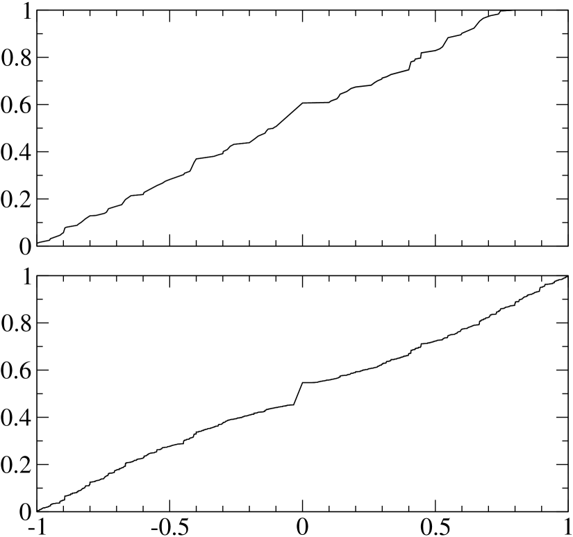
Figure 2: Comparison of the conformations produced by WH and by standard reptation for an isolated polymer of size $N=50$ at $T=2$. Both figures show two curves superimposed, but they are indistinguishable. Top: the integrated distributions of $\cos\theta$ with $\theta$ the angle between two successive bonds. Bottom: the integrated distributions of $\sin\phi$ with $\phi$ the (torsion) angle between a bond and the plane defined by the two preceeding bonds.

To check the correctness of the implementation, we used our program to simulate isolated chains of different lengths with attractive interactions near the $\Theta$-temperature (namely $T=2$). This is the most sensitive point to check that the conformation of the chain is correctly sampled, since it is where the fluctuations and the temperature dependence are the largest. First we reproduced the measurements of the $\Theta$-temperature done by Wilding et al. [13] and found fully compatible results (namely $T_{\Theta}=2.03(3)$ to be compared with $T_{\Theta}=2.02(2)$). Moreover we compared the distributions of the bond-bond and torsion angles with the ones given by standard reptation. The results are shown on figure 2. Both algorithms give the same results (within statistical error bars, here roughly $0.1\%$) and the curves, on top of one another, are indistinguishable. Note that the roughness of the curves is no noise, it is due to the discreteness of the model.

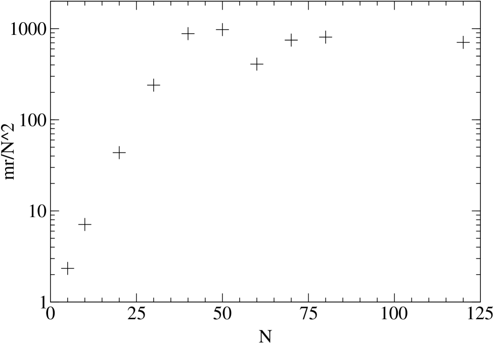
Figure 3: The number of accepted elementary steps required to achieve a complete WH move is $O(N^{2})$.

All the following benchmarks are made using a mixture of polymers of length $N$ at density $1/2$ in the BFM at infinite temperature. For these parameters, our computer (a Pentium III at 500 MHz) achieve $1.3\ 10^{6}$ elementary steps per second with an acceptance rate $r\simeq 8.5\%$. Note that our implementation also works at finite temperature and is thus slower than an implementation optimised for the infinite temperature case.

First, we have claimed that our algorithm is able to completely displace a polymer in time $N^{2}$. This is a reasonable assumption since it is the time required by an unbiased random walk to cover a distance $N$ and this corresponds to a complete WH move. But this must be tested numerically since the random walk actually done is strongly influenced by density fluctuations. We note $m$ the mean number of elementary steps required to achieve one complete WH move (many failed and partial moves may also happen in between) and $mr$ is the corresponding number of accepted elementary steps. The values of $mr/N^{2}$ are shown as a function of $N$ in figure 3, they clearly show that for large $N$, we have

$$m=\frac{\alpha}{r}N^{2},$$ (9)

with $\alpha\simeq 800$. To achieve a complete move on our computer, we thus need around $7.\ 10^{-3}N^{2}$ seconds for a long polymer (and less for a smaller one). As could be expected, the value of $\alpha$ decreases at lower density, for example at density $0.1$, $\alpha\simeq 1.8$ (and $r\simeq 67.5\%$).

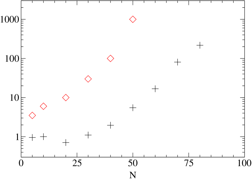
Figure 4: CPU time ratios between CB and WH as a function of $N$. Crosses are time ratios for completely displacing a polymer (time to accept a CB move/time to do a complete WH move). Diamonds are relaxation time ratios (see equation 10).

What our algorithm can do is very similar to CB, so it is interesting to do the comparison. The CB with which we compare tries to erase a polymer completely and to recreate it somewhere else, for each monomer it checks the 108 possible bonds and chooses an allowed one (not already occupied) and computes the associated weight. On our computer, we can do $7.10^{4}$ such elementary steps per second (one needs $N$ of them for a whole CB move). As for WH, our CB implementation also works at finite temperature and is thus slower than it should for the infinite temperature case. Note that one could also use a CB implementation which does not check all the 108 bonds (say 10 or 20). In this case the elementary steps are accordingly faster but the overall acceptance rate decreases much faster with $N$.

In figure 4, we show the ratios of time required by both algorithm to completely displace a polymer (an accepted CB move and a complete WH move). From this point of view, the algorithms are more or less equivalent at small $N$, and WH becomes exponentially better at large $N$. In this first comparison we did not take into account the fact that WH also relaxes the system when it does a partial move. So we measured the relaxation time of the end-to-end vector $\mathbf{R}(t)$, namely:

$$\tau=\frac{1}{\langle\overline{\mathbf{R}^{2}}\rangle}{\int\langle\mathbf{R}(0)\cdot\mathbf{R}(t)\rangle\mbox{d}t}.$$ (10)

The ratios of those times are also shown on figure 4, clearly WH is much faster than CB. On the other hand, at a lower density, CB is more efficient for the small values of $N$ (for example at density 0.1 and at $N=40$, CB is only 3 times slower than WH instead of 100 times slower), but CB stays exponentially slower at large $N$. See below how one could take advantage of a faster CB for small $N$.

Finally this comparison was done on a lattice, this gives a big advantage to CB since off-lattice CB implementations require a large number of energy computations which are much longer than on a lattice. Moreover, reptation is hampered by the lattice since it can get blocked much more easily than off-lattice. We thus think that WH should be even better for continuous models.

Our WH method is reminiscent of the extended ensemble method introduced by Escobedo and de Pablo [14, 15]. But in their method, the elementary steps are CB moves that move $k$ monomers at a time. Moreover the intermediate configurations are also sampled giving rise to extended ensembles with configurations where a polymer is incomplete or split into two pieces. Since they relax the whole system between each elementary step the time to deal with one polymer is

$$m^{\prime}=\frac{\alpha^{\prime}V}{r^{\prime}}\left(\frac{N}{k}\right)^{2},$$ (11)

with $V$ the number of particles in the system and $\alpha^{\prime}$ and $r^{\prime}$ the equivalent of $\alpha$ and $r$ in equation 9. Here $r^{\prime}\propto\exp(-k/k_{0})$ and there is an optimal value for $k$ (namely $k=2k_{0}$). With our parameters $k_{0}\simeq 4.5$ and $r^{\prime}\simeq 3\%$, so even if $\alpha^{\prime}<\alpha$, $V/k^{2}$ is very large.

Finally, WH has one feature which may be undesirable. The execution time for one move has huge fluctuations (that explains the fluctuations in figure 3). A move can be very fast (for example a failed move) but it can also last a few seconds (and exceptionally a few minutes for long chains). In a simple simulation that is no problem, since only the average time is relevant. But in a parallel computation, where each processor waits after the slowest one, this can become a real difficulty. A first solution is to do a lot of WH moves between two synchronisations, thus averaging the fluctuations. Another one is to set a limit to the number of elementary steps which can be done in one move (say $10m$). If this threshold is exceeded, the move is rejected and the polymer is restored to its initial state.

4 Variations

Let us first see algorithmic refinements to WH. First, in the case of an off-lattice simulation one may wish to draw the polymer bonds out of a non-uniform $P_{B}$ distribution. In particular one may want to draw the bond length around a certain favourable value. In such a case it is necessary to add a correcting weight to the Metropolis rule to recover equation 5 (as done for normal reptation). Then one can check that these correcting weights raise the correct overall correction term and equation 8 still holds so the algorithm is still correct. More generally, as soon as one wants to modify the WH algorithm, one should check that the cancellations still occur, in particular for $i=1$ and $i=n$.

In the original reptation method [3] the direction of the reptation is changed only when a move is rejected and not drawn randomly at each step as we propose here. Nothing prevents to do the same in WH (the proof just gets a little more complicated). At very low density this can improve the speed by a factor 2 or more because successive steps are done in the same direction. But at high density, it changes essentially nothing.

As explained in the previous section, CB can be more efficient at small $N$ than WH (at low density or when we do not check all the 108 bonds at each step). Then, as done in the “extended ensemble” method, one can use CB as the elementary step, moving $k$ monomers at a time and we then have (with notation of the previous section)

$$m=\frac{\alpha}{r^{\prime}}\left(\frac{N}{k}\right)^{2},$$ (12)

and the CPU time is proportional to $km$ (the optimal value of $k$ is now $k=k_{0}$). This is faster than the original WH if $kr^{\prime}/r>K$ with $K$ the CPU time ratio to do one elementary move with both methods (here $K\simeq 19$). Note that we have supposed that $\alpha$ does not change which is not clear. Finally one of the interesting point in WH is the ease of programming, this is lost in this variation.

Let us now see how WH can be extended. First, how to do grand canonical moves. These moves can be of three different kinds: (i) to move a polymer from one simulation box to another one; (ii) to remove one polymer from a box; (iii) to insert a new polymer in a box. The first one is very easy to do, WH applies directly and one can eventually add a chemical potential for each monomer depending on the box. For (ii) and (iii), one proceeds more or less as for CB. The algorithm has to be modified, the reptation steps are made between the simulation box and some kind of black box without geometry where the monomer have a given chemical potential. The $P_{B}$ and $P_{P}$ no longer completely cancel (the steps toward the black box do not require a random draw) and for an inserting move and the corresponding removing move, equation 8 becomes

$$\frac{P(S)}{P(\overline{S})}=e^{-\beta(E_{n}-E_{0})}P_{P}P_{B}^{N-1}.$$ (13)

The new factor is a constant which can be absorbed in the chemical potential (exactly as the weight with CB). This factor is exactly the probability for choosing a particular configuration of the polymer. We did not perform tests for the grand canonical moves, but we expect them to behave as described in the previous section.

Figure 5: A complete modified WH move. The letters represent different kind of monomers in a hetero-polymer. Note how in the intermediate configurations, monomer F has disappeared and monomer C is present twice.

Very often CB is not used to remove and insert a whole polymer, but is applied only on a part of it. Such a thing can also be done with WH, provided we perform a little modification (see figure 5). At the first step of the algorithm, instead of choosing a random position, the monomer is randomly bound to another non-end monomer of the same polymer. After this, WH proceeds as before until the polymer is linear again. Note that in the case of a hetero-polymer, the monomer that goes through the hole may be replaced by another one, so that the polymer has kept its structure at the end (see figure 5). This modified move is probably less efficient than the original one for the same number of monomers, since the new growing branch is going to encounter an already densely occupied region (the old branch being also there). Moreover the original WH is also able to move parts of the polymer (with partial moves), so it is perhaps better to use the original move. The modified move can in any case be useful for branched polymers.

Figure 6: The order in which the monomers enter the hole (left), and leave it (right) for a branched polymer.

Finally one can also extend the original WH to branched polymers. The basic idea stays the same: a random walk through a set of non-valid configurations where the polymer is split into two pieces. But it cannot use simple reptation because of the branching points. One way to achieve this is to make the monomers get out of the hole in a different order as they enter it. See figure 6 for an example. As in the previous paragraph, during the move, certain monomers may be present twice whereas others are no longer there.

5 Discussion and Conclusions

The wormhole move (WH) presented here is a new kind of Monte Carlo move for polymer simulations. It can completely displace a polymer in time $O(N^{2})$ even at high density ($1/2$ in the bond fluctuation model). It is based on reptation steps and is thus quite easy to program. It is nevertheless very flexible since it works on hetero-polymers, allows grand canonical moves (insertions and deletions of polymers) and can be adapted to branched polymers.

What is this new method good for ? Essentially, it is meant to replace configurational bias (CB). The wormhole move can in fact do whatever CB does, and it does it faster. As CB, it can destroy, create or displace a polymer, but CB works in time $O(e^{\gamma N})$ whereas WH works in time $O(N^{2})$. Thus, exception made of the case of short polymers at low density, it is always better to use WH instead of CB. In the case of short polymers at low density, it is probably better to use WH as well, since this case is anyway an easy one which requires short computation time and WH is relatively easier to program.

On the other hand, the aim of WH is not to replace the standard reptation method or to compete with it. It simply does something different. Typically standard reptation is to be preferred in the case of linear homo-polymers with small density fluctuations (i.e. when it is not important to be able to rapidly displace a polymer between two distant positions). In the other cases, where one would have used CB, one should use WH. There are essentially two main cases: (i) if reptation is not applicable, in particular to do grand canonical moves or to simulate hetero-polymers; (ii) in the case of large density fluctuations (typically when more than one phase is present) where one wants to rapidly relax the density by displacing polymers over large distances.

We expect this new method to become widely used since it is easy to program and very efficient. At the moment, it is used to simulate dense random copolymer mixtures [16].

The author acknowledges M. Müller, L. G. MacDowell, A. Yethiraj and K. Binder for fruitful discussions.

References

- 1 Monte Carlo and Molecular Dynamics Simulations in Polymer Science, K. Binder, ed., (Oxford University Press, New York, 1995).
- 2 N. Madras and A. Sokal, J. Stat. Phys. 50, 109 (1988).
- 3 F. T. Wall and F. Mandel, J. Chem. Phys. 63, 4592–4595 (1975).
- 4 J. I. Siepmann and D. Frenkel, Mol. Phys. 75, 59–70 (1992).
- 5 D. Frenkel, G. C. M. A. Mooij, and B. Smit, J. Phys.: Condens. Matter 4, 3053–3076 (1992).
- 6 F. A. Escobedo and J. J. de Pablo, J. Chem. Phys. 102, 2636–2652 (1995).
- 7 S. Consta, N. B. Wilding, D. Frenkel, and Z. Alexandrowicz, J. Chem. Phys. 110, 3220–3228 (1999).
- 8 K. Hukushima and K. Nemoto, J. Phys. Soc. Jpn. 65, 1604–1608 (1996).
- 9 A. M. Ferrenberg and R. H. Swendsen, Phys. Rev. Lett. 61, 2635–2638 (1988).
- 10 P. Grassberger, Phys. Rev. E 56, 3682–3693 (1997).
- 11 I. Carmesin and K. Kremer, Macromolecules 21, 2819–2823 (1988).
- 12 H.-P. Deutsch and K. Binder, J. Chem. Phys. 94, 2294–2304 (1991).
- 13 N. B. Wilding, M. Müller, and K. Binder, J. Chem. Phys. 105, 802–809 (1996).
- 14 F. A. Escobedo and J. J. de Pablo, J. Chem. Phys. 103, 2703–2710 (1995).
- 15 F. A. Escobedo and J. J. de Pablo, J. Chem. Phys. 105, 4391–4394 (1996).
- 16 J. Houdayer and M. Müller, in preparation.