Evidence for Slow Velocity Relaxation in Front Propagation in Rayleigh-Bénard Convection

Abstract

Recent theoretical work has shown that so-called pulled fronts propagating into an unstable state always converge very slowly to their asymptotic speed and shape. In the the light of these predictions, we reanalyze earlier experiments by Fineberg and Steinberg on front propagation in a Rayleigh-Bénard cell. In contrast to the original interpretation, we argue that in the experiments the observed front velocities were some 15% below the asymptotic front speed and that this is in rough agreement with the predicted slow relaxation of the front speed for the time scales probed in the experiments. We also discuss the possible origin of the unusually large variation of the wavelength of the pattern generated by the front as a function of the dimensionless control parameter.

I Introduction

Although the propagation of a front into an unstable state plays an important role in various physical situations ranging from the pearling instability [1, 2] to dielectric breakdown [3], detailed experimental tests of the explicit theoretical predications, especially those for the velocity of so-called “pulled” fronts are scarce. One of the reasons lies in the difficulty in preparing the system in the unstable state.

If the initial front profile is steep enough the propagating front converges to a unique shape and velocity. Theoretically, one distinguishes two regimes for front propagation into unstable states: the so-called “pushed” regime, where the front is driven by the nonlinearities and the so-called “pulled” regime where the asymptotic velocity of the propagating front, $v_{as}$, equals the spreading speed $v^{*}$ of linear perturbations around the unstable state: $v_{as}=v^{*}$. Pushed fronts are by definition those for which the asymptotic speed $v_{as}$ is larger than $v^{*}$: $v_{as}>v^{*}$. It is thus as if a “pulled” front is literally “pulled” by the leading edge whose dynamics is driven by linear instability of the unstable state [4, 5, 6, 7]; the nonlinearities merely cause saturation behind the front. We focus here on the experimental tests of the dynamics of such pulled fronts; since $v^{*}$ is determined by the equations linearized about the unstable state, the front velocity of pulled fronts can often be calculated explicitly, even for relatively complicated situations.

There have been two experiments aimed at testing the predictions for the speed of pulled fronts. Almost 20 years ago Ahlers and Cannell [8] studied the propagation of a vortex-front into the laminar state in rotating Taylor-Couette flow. The measured velocities were about 40% smaller than expected from the theoretical predictions. A few years later, however, Fineberg and Steinberg (FS) [9] published data which appeared to confirm the expected velocity in a Rayleigh-Bénard convection experiment to within about 1%. The issue then seemed to be settled when it was also shown that the discrepancy observed by Ahlers could be traced back to slow transients [10].

The theoretical developments of the last few years give every reason to reconsider the old experiments by FS: It has been shown [7] that the convergence of the velocity of pulled fronts is always very slow, in fact with leading and subleading universal terms of ${\mathcal{O}}(1/t)$ and ${\mathcal{O}}(1/t^{3/2})$ with prefactors which follow from the linearized equation. This slow relaxation implies that it will in general be very difficult to measure the asymptotic front speed to within a percent or so in any realistic experiment. Hence, from this new perspective, the proper question is not why in the Taylor-Couette experiment the measured velocity was too low, but why apparently in the Rayleigh-Bénard experiment of FS the asymptotic front speed was measured.

The main purpose of this paper is to address this issue, and to reanalyze the experiments in the light of the present theory. We will conclude that the data of FS actually do show signs of the predicted power law convergence of the front velocity to an extrapolated asymptotic value which is about 15% larger than their transient value. This of course implies that there is then a discrepancy of order 15% between the value of $v_{as}=v^{*}$ as extrapolated from their data, and the one claimed in the original experiments. We will argue that the most likely reconciliation of the two results is that the value of the correlation length $\xi_{0}$ in the experimental cell of FS is somewhat larger than the theoretical value used by FS to interpret their data.

Of course, only new experiments can settle whether the interpretation we propose is the correct one. We do consider new experiments along the lines of FS in fact very desirable, not so much as they might settle the numerical value of the velocity, but more because they hold the promise of being the first accurate experimental test of the universal power law relaxation of pulled fronts.

In section II we will first summarize the relevant theoretical predictions for the velocity of pulled fronts. Then we will discuss the experiments of FS in the light of these results in section III, where we will also reanalyze their data. Finally, in section IV we turn to a brief discussion of the wavenumber of the pattern selected by the front. Here, the results of FS were not quite consistent with the predictions for the asymptotic wavenumber from the Swift-Hohenberg equation. As we shall discuss, the wavelength of the pattern is affected by various effects which are not easily controlled, but the most likely interpretation of the data of FS is that they did not observe the asymptotic wavelength behind the front, but the local wavenumber in the leading edge of the front. Indeed it is in general difficult to test the theory by studying the asymptotic pattern wavelength and the convergence to the asymptotic value experimentally.

II Summary of theoretical predictions

A Asymptotic speed and power law convergence

Just above the onset of a transition to stationary finite wavelength patterns, for small dimensionless control parameters $\epsilon$ the slow dynamics on length scales larger than the wavelength of the pattern can be described by the Ginzburg-Landau amplitude equation [11, 12]

$$\tau_{0}\partial_{t}A=\epsilon A+\xi_{0}^{2}\partial^{2}_{x}A-g|A|^{2}A~{}.$$ (1)

The time scale $\tau_{0}$ and length scale $\xi_{0}$ as well as the nonlinear saturation parameter $g$ depend on the particular system under study.

The asymptotic spreading speed $v^{*}$ of linear perturbations around the unstable state is in general obtained from the linear dispersion relation $\omega(k)$ of a Fourier mode $e^{-i\omega t+ikx}$ through

$$\left.\frac{\partial{\rm Im}\omega}{\partial{\rm Im}k}\right|_{k^{*}}-v^{*}=0,~{}~{}\left.\frac{\partial{\rm Im}\omega}{\partial{\rm Re}k}\right|_{k^{*}}=0,~{}~{}\frac{{\rm Im}\omega(k^{*})}{{\rm Im}k}=v^{*}.$$ (2)

This yields for the Ginzburg-Landau equation [13]

$$v^{*}=2\epsilon^{1/2}\xi_{0}\tau_{0}^{-1}~{}.$$ (3)

and

$$\mu^{*} \equiv \mbox{Im}k^{*}=\sqrt{\epsilon}/\xi_{0}~{},$$ (4)

$$D \equiv \frac{1}{2}\left.\frac{\partial^{2}{\rm Im}\omega}{(\partial{\rm Im}k)^{2}}\right|_{k^{*}}=\frac{\xi^{2}_{0}}{\tau_{0}}~{}.$$ (5)

In the experiments with which we will compare, the scaled velocity

$$\tilde{v}=v\frac{\tau_{0}}{\xi_{0}\sqrt{\epsilon}}$$ (6)

is often used. According to (3), for a pulled front the asymptotic value $\tilde{v}_{as}=2$.

The above results were known in the eighties, at the time when the experiments were done. The crucial insight of the last few years is the finding that the convergence or relaxation towards the asymptotic velocity $v^{*}$ of pulled fronts is always extremely slow: the general expression for the time dependent velocity $v(t)$ emerging from steep initial conditions (i.e., decaying faster than $e^{-\mu^{*}x}$) is given by [7, 13]

$$v(t)=v^{*}-\frac{3}{2\mu^{*}t}+\frac{3}{2\mu^{*2}t^{3/2}}\sqrt{\frac{\pi}{D}}+{\mathcal{O}}(t^{-2})~{}.$$ (7)

For the case of the Ginzburg-Landau amplitude equation, we then have

$$\tilde{v}(t)=2-\frac{3}{2\epsilon t/\tau_{0}}+\frac{3\sqrt{\pi}}{2(\epsilon t/\tau_{0})^{3/2}}+\cdots$$ (8)

It is important to stress that the above expression for $v(t)$ is exact but asymptotic — this is illustrated by the fact that at time $\epsilon t/\tau_{0}=\pi$ the subdominant $t^{-3/2}$ term is equal to the first correction term of order $t^{-1}$ in absolute value, but of opposite sign. Thus, although for any sufficiently long time $t$, the above expression will always become accurate, at any finite time, however, the expression might only yield a good estimate. In fact, in practice one usually has to go to dimensionless times $\epsilon t/\tau_{0}$ of order 10 or larger for the asymptotic expression to become accurate, while for dimensionless times $\varepsilon t/\tau_{0}$ in the range 3 to 10 the first correction term yields a reasonable order-of-magnitude estimate [7]. As we shall see below, in the Rayleigh-Bénard experiments [9] the maximum dimensionless time $\epsilon t/\tau_{0}$ that can be probed is about 3 to 4. In comparing with experiments and in making order of magnitude estimates, we will therefore only use the first correction term. Finally it is important to realize that after how long a time these expressions become really accurate, depends also on the initial conditions.

B Dependence on initial conditions

In order to illustrate how accurate these expressions are in practice, we numerically integrate the real Ginzburg-Landau equation starting with an exponentially decaying initial condition with steepness $\mu$ [13]: $A(x,t=0)=ae^{-\mu x}$. The result is shown in Fig. 1 for various values of $\mu$. We see that initially the velocity falls off quickly and then approaches the asymptotic velocity from below, and that the asymptotic expression (8) in practice does yield a reasonable estimate of the time dependent velocity for values of the scaled time of order 3 and larger.

We also note that the theoretical analysis shows that for initial profiles falling off exponentially with steepness $\mu<\mu^{*}$, the asymptotic velocity lies above $v^{*}$ and is given by $v_{as}(\mu)=\mu+\frac{1}{\mu}$. The dotted line in Fig. 1 shows an example of a case with $\mu$ slightly less than $\mu^{*}$, for which $\tilde{v}_{as}=2.05$. In this case, the time-dependent scaled velocity is approximately equal to 2 at times of order 3 to 4.

In the experiments, the typical protocol was to simultaneously increase the heat flux from an initial state at $\epsilon_{i}<0$ (with a typical value of $\epsilon_{i}=-0.015$) to a supercritical value $\epsilon_{f}$, and switching on the end heater. A rapid convergence to the asymptotic velocity due to special initial conditions with $\lambda\approx\lambda^{*}$ would have required setting $\epsilon_{i}\approx-\epsilon_{f}$ for all $\epsilon_{f}$ and would probably also have required switching on the end heater before the value of $\epsilon$ was changed, so that effectively at the end a convection pattern was prepared whose amplitude decayed exponentially into the bulk. Thus, it is theoretically possible to select special initial conditions so as to get a scaled velocity around 2 at some finite time, but the finetuning necessary to do so is so sensitive that we consider it very unlikely that experimental observations done over a range of values of $\epsilon$ are due to initial condition effects. As stressed before, only new experiments can completely rule out this possibility, however.

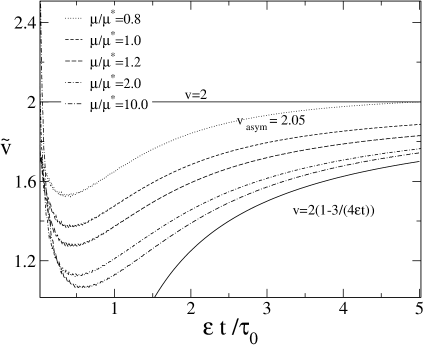
FIG. 1.: Velocity of fronts propgating propgating into the unstable state $A=0$ of the real Ginzburg-Landau equation with exponentially decaying initial conditions $A=\sqrt{\epsilon/g}\>e^{-\mu x}$. The velocity is obtained by tracing the position of the point where $A$ reaches half its asymptotic value. Since $\epsilon$ and $\xi_{0}$ just set the length and time scale, $\tilde{v}(t)$ plotted as a function of the scaled time $\epsilon t/\tau_{0}$ is parameter-independent. Different initial conditions or tracing a different value of $A$ to determine the velocity yield different transient behavior, but for sufficiently steep initial conditions, all curves converge to the analytic formula for late times.

III Reexamination of the Rayleigh-Bénard fronts

In the long quasi-one-dimensional Rayleigh-Bénard cell of FS [9] the front propagation was initiated by simultaneously increasing the heat flux to a supercritical value $\epsilon>0$ ($\epsilon=\frac{\Delta T}{\Delta T_{c}}-1$) and switching on a heater at the ends of the long cell. A vortex front is induced near the this heated end-wall and the propagation of this front into the unstable conductive state is then studied. Thin fins were attached to the long sides of the cell to avoid both induction of long rolls and pinning. Both because of the fact that the initial perturbation was caused by heating at the end and because the state before bringing the temperature difference beyond its critical value was unrelated to the final value of $\epsilon$, there is every reason to believe that the experimental protocol did not create any special initial conditions that can not be considered sufficiently steep or localized.

As FS point out, since the front velocity $v^{*}$ grows as $\sqrt{\epsilon}$ while the growth rate in the bulk grows as $\epsilon$, fronts can only be observed and in fact dominate the dynamics for small enough $\epsilon$. In practice the pattern could be distinguished from the bulk noise up to a time $t_{bg}=n\tau_{0}\epsilon^{-1}$ where the numerical factor $n$ is of order 3–4. This determines some upper limit $\epsilon_{0}$ on $\epsilon$ for which the front can advance of the order of $(1/m)$th of the cell length $l$ before bulk growth takes over:

$$\epsilon_{0}=\left(\frac{\tilde{v}\xi_{0}mn}{l}\right)^{2}.$$ (9)

Let us now estimate, using our analytical estimate (8), the relative importance of the correction term at the latest times of order $t_{bg}=n\tau_{0}\epsilon^{-1}$ at which measurements can be taken. Substitution gives

$$\tilde{v}(t_{bg})\approx 2\left(1-\frac{3}{4n}\right).$$ (10)

Thus, for the latest time accessible in the experiment, we obtain with the empirical experimental value $n=$3–4 a velocity which is of order $20\pm 5\%$ below the asymptotic value. Although the asymptotic formula may not be accurate yet at such early times, the numerical results of Fig. 1 lead one to expect corrections of the same order of magnitude: these times also correspond to scaled times of order $n$ in the numerical simulation plots of Fig. 1, and as we have seen, over this time range, the velocity is also suppressed by about 15% relative to the asymptotic value. Hence, by any reasonable estimate, the slow relaxation can not be negligible in the experiments!

As stated in the introduction, FS quoted a measured velocity $\tilde{v}=2.01\pm 0.02$ for their experiments, contrary to our expectation that their scaled velocity should have been in the neighborhood of 1.7. According to the theoretical results, one should expect to get to within 1% of the asymptotic velocity only around a dimensionless time of order 100!

In our view, the most plausible explanation for the origin of this discrepancy is that the value $\xi_{0}$ was actually larger in the experiments than the value used in the analysis. The value of $\tau_{0}$ was experimentally confirmed to be very close to the theoretical value [14, 15]. For $\xi_{0}$, however, the theoretical value was used without independent experimental check [14]. Because of the special design of the cell with side-fins to create one-dimensional patterns, a different value of $\xi_{0}$ might not be unexpected. In fact, an indication that $\xi_{0}$ in the experiments was larger than the theoretical value used in the analysis, comes from the observation of FS that the value of the wavelength at onset was 13% larger than the theoretical value. This might indicate that all lengths in the experiments are a factor 1.13 larger than the theoretical values, and this is precisely the factor needed to reconcile the front data with the theoretical expectations! One should keep in mind, though, that $\xi_{0}$ is determined by the the curvature of $\epsilon$ versus $k$ tongue around the critical wavenumber, and that it is not guaranteed that both are changed by the same factor; only independent measurements can fully settle this issue.

We now show that a reanalysis of the data of FS actually gives quite convincing evidence for slow convergence effects in the experimental fronts.

FS measured the velocity by comparing the front with itself at various time intervals, by appropriately shifting the traces back. This yielded a set of points in the $\Delta x$, $\Delta t$ plane which appeared to lie on a straight line. However a possible relaxation of the velocity was masked since points from early and later times will approximately fall in the same place in the plane, and because the front shape also has an asymptotic $1/t$ relaxation. We therefore have tried to reanalyze the raw data of figure 2 from the FS paper; this space-time plot of a propagating from is reproduced in the top panel of our Fig. 2. We define the position of the front as the point where the interpolation of the maxima of the profile equals some fraction of its maximum in the bulk (we chose 0.4). Our data for $\tilde{v}(t)$ obtained this way are shown in the lower panel of Fig. 2. Whereas the local velocity initially slightly decreases, an increase for dimensionless times larger than 0.5 is evident. We stress that this qualitative behavior is independent of the choice of the parameters. In order to compare quantitatively to the predictions for the relaxation, we have used the value for $\tau_{0}$ given by FS but increased the value of $\xi_{0}$ by 13% on the basis of the argument given above. Clearly, with this choice, the data are certainly consistent with the analytical as well as numerical estimates of the velocity relaxation — in fact, in a way the data are the first experimental indications for the universal power law relaxation of pulled fronts [17].

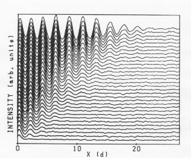
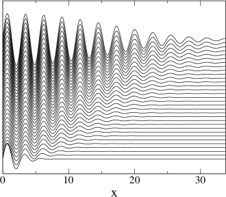
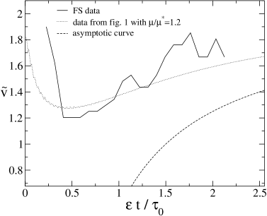
FIG. 2.: Top panel: shadowgraph trace of a propagating front in the experiments of FS for $\epsilon=0.012$ [14]. The time difference between successive traces is 0.42 $t_{v}$, where $t_{v}$ is the vertical diffusion time in the experiments, and the distances are measured in units $d$ (the cell height). (from [9]). Middle panel: similar data obtained from numerical integration of the Swift-Hohenberg equation also at $\epsilon=0.012$ starting with a localized initial condition. The time difference between successive traces corresonds to 0.42 $t_{v}$. Bottom panel: Velocity versus time in the experiment, as obtained by interpolating the maxima of the traces in the top panel, as explained in the text. The dashed line shows the analytical result (8) and the dotted curve the result of the amplitude equation simulation of Fig. 1 with $\mu/\mu^{*}=1.2$. Note that the curves are not fitted, only the absolute scale is affected by adjusting $\xi_{0}$.

IV Relaxation of wavelength

FS also studied the problem of the selection of the wavelength $\lambda$. As we discussed before, the actual value of the wavelength $\lambda_{c}$ of the patterns is at criticality about 13% off from the theoretical value; however, we are not interested here in the absolute value, but in the relative variation of $\lambda_{c}/\lambda$.

The difficulty of comparing theory and experiment on the variation of the wavelength is that the only theorically sharply defined quantity is the wavelength sufficiently far behind the front, $\lambda_{as}$, and that one has to go beyond the lowest order Ginzburg-Landau treatment to be able to study the pattern wavelength left behind. E.g., if we use a Swift-Hohenberg equation for a system with critical wavenumber $k_{c}$ and bare correlation length $\xi_{0}$,

$$\partial_{t}u=-\frac{(\xi_{0}k_{c})^{2}}{4}\left(1+\frac{1}{k^{2}_{c}}\frac{\partial^{2}}{\partial x^{2}}\right)^{2}u+\epsilon u-u^{3},$$ (11)

then a node counting argument [4, 6] yields for the asymptotic wavelength $\lambda_{as}$ far behind the front [6]:

$$\frac{\lambda_{c}}{\lambda_{as}} = \frac{3\left(3+\sqrt{1+24\epsilon/(k_{c}^{2}\xi_{0}^{2})}\right)^{3/2}}{8\left(2+\sqrt{1+24\epsilon/(k_{c}^{2}\xi_{0}^{2})}\right)}$$ (12)

$$\approx 1+\epsilon/(2k_{c}^{2}\xi_{0}^{2})~{}~{}~{}~{}(\epsilon\ll 1)~{}.$$ (13)

In the Rayleigh-Bénard experiments, $k_{c}\approx 2.75/d$, where $d$ is the cell height; the theoretical value is $\xi_{0}=0.385d$, so if our conjecture that the value is some 15% larger is correct, we get $\xi_{0}\approx 0.44d$. This then gives

$$\frac{\lambda_{c}}{\lambda_{as}}\approx 1+0.34\epsilon.$$ (14)

As we stressed already above $\lambda_{as}$ is the wavelength far behind the front; for a propagating pulled front, there is another important quantity which one can calculate analytically, the local wavelength $\lambda^{*}$ measured in the leading edge of the front. For the Swift-Hohenberg equation, one gets for this quantity[6, 16]

$$\frac{\lambda_{c}}{\lambda^{*}} = \sqrt{1+\frac{1}{4}\left(\sqrt{1+24\epsilon/(k^{2}_{c}\xi_{0}^{2})}-1\right)}$$ (15)

$$\approx 1+\frac{3\epsilon}{2k_{c}^{2}\xi_{0}^{2}}~{}~{}~{}~{}~{}(\epsilon\ll 1)~{}~{}~{}~{}$$ (16)

$$\approx 1+\epsilon,$$ (17)

where in the last line we have used the experimental values.

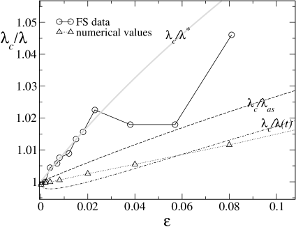
FIG. 3.: The selected wave number $\lambda_{c}/\lambda$ as function of $\epsilon$. The data points of FS are denoted by circles, our numerical results on the Swift-Hohenberg by triangles. The dashed lines shows the prediction for the asymptotic wavelength, the dashed-dotted line shows the analytic result with relaxation terms at $t=6\tau_{0}/\sqrt{\epsilon}$ [16] and the grey line shows the result for the local wavelength in the leading edge.

Let us now discuss the experimental findings in the light of these results. In Fig. 3 we show both the experimental values of $\lambda_{c}/\lambda_{exp}$ as determined experimentally by FS, and results for the Swift-Hohenberg equation with the value (14) relevant for the experiments.
    (i) For small $\epsilon$, the experimental values are roughly linear in $\epsilon$, but when a fit is made over the whole range of $\epsilon$ values studied, a square root behavior, as proposed by FS, would probably be better.
    (ii) The experimental values for the wavelength ratio deviate about a factor of 3 from the theoretically expected value for the ratio far behind the front, $\lambda_{c}/\lambda_{as}$.
    (iii) Just like the front speed converges very slowly to the asymptotic value, so does the local value of the wavelength behind the front [16]. The relaxation of the velocity is plotted with a dashed-dotted line in Fig. 3 for times about $6\tau_{0}/\sqrt{\epsilon}$, which is the time it takes for a front to propagate to close to the center of a system about as large as the experimental cell. Clearly, the wavelength ratio due to slow relaxation lies below the asymptotic value, and hence further away from the experimental data for small $\epsilon$. Also, numerical results for the wavelength of the fourth “roll” measured at the same time (indicated by the dotted line, lie below the asymptotic curve.
    (iv) FS have measured the wavelength for very small values of $\epsilon$, down to $4\;10^{-4}$. However, already for values as small as 0.01, the coherence length $\xi=\xi_{0}/\sqrt{\epsilon}$ is about $2\lambda_{c}$ in the experiments. The total front width is several times this number, and for even smaller values of $\epsilon$ the front width is even smaller. Since the total experimental cell was about $12\lambda_{c}$ long in the experiments, it is clear that over much of the small $\epsilon$ range, one would not expect to see well-developed fronts in the experiments. In other words, it is very unlikely that over the experimental range of $\epsilon$-values, one has a chance to measure $\lambda_{as}$ of a well-developed pattern behind a front.
    (v) The grey line in the plot shows our analytical result for the wavelength ratio in the leading edge of the front. Clearly, this line follows the data for small $\epsilon$ quite well. In view also of point (iv) above that it will be hard to obtain well-developed fronts for small $\epsilon$, we propose as a tentative explanation of the data that in the small $\epsilon$ range, one actually measures the emergent roll pattern associated with the leading edge of a front. Of course, only new experiments can decide on the validity of this suggestion.
    (vi) We mention that the variation of the wavelength ratio with $\epsilon$ depends also on the third order derivative term in the expansion of the dispersion relation around the critical wavenumber. This term is not modeled correctly in the Swift-Hohenberg equation, but may have to be taken into account in a full comparison of theory and experiment.
    (vii) We finally mention that in the experiments there was an up-down asymmetry in the rolls. We have investigated whether this could be a source of the discrepancy between the asymptotic wavelength ratio and the observed one, by studying a Swift-Hohenberg equation with a symmetry-breaking quadratic term. However, with this term, the wavelength ratio apears to decrease away from the experimental values.

V Conclusion

It was recently discovered that quite generally pulled fronts relax very slowly to their asymptotic velocity. Comparison of the experimental data for the velocity with numerical simulations and analytical estimates give, in our view, evidence that these experiments provide clear signs of the presence of such slow relaxation effects, although the time scales that can be probed experimentally are too short to test the general power law relaxation. Theoretically the only other viable option to reconcile theory with the interpretation originally proposed [9] is that somehow special initial conditions created an initial convection profile with precisely the right spatial decay into the bulk. As we discussed in section III, in our view this is an unlikely interpretation, but only new experiments can settle this issue completely.

While measurements of the wavelength of the pattern generated by a front are even more difficult to interpret than those of the velocity, our analysis indicates that in the small-$\epsilon$ regimes a well-developed front does not fit into the experimental cell, and that as a result one probes the local wavelength in the leading edge of the front rather than the well-developed asymptotic wavelength behind it. The analytical estimates are consistent with this suggestion.

We hope that this work will trigger new experimental activity to investigate these issues — experiments along these lines hold the promise of being the first ones to see the universal power law relaxation of pulled fronts.

VI Acknowledgement

We are grateful to Jay Fineberg and Victor Steinberg for correspondence about their work and about the issue discussed in this paper. WvS would also like to thank Guenter Ahlers for urging him to analyze to what extent slow convergence plays a role in the Rayleigh-Bénard experiments. JK is grateful to the ‘Instituut-Lorentz’ for hospitality.

REFERENCES

- [1] R. Bar-Ziv and E. Moses, Phys. Rev. Lett. 73, 1392 (1994).
- [2] T. R. Powers and R. E. Goldstein, Phys. Rev. Lett. 78, 2555 (1997).
- [3] U. Ebert, W. van Saarloos and C. Caroli, Phys. Rev. E 55, 1530 (1997).
- [4] G. Dee and J. S. Langer, Phys. Rev. Lett. 50, 383 (1985).
- [5] E. Ben-Jacob, H. Brand, G. Dee, L. Kramer and J. S. Langer, Physica 14D, 348 (1985).
- [6] W. van Saarloos, Phys. Rev. A 39, 6367 (1989).
- [7] U. Ebert and W. van Saarloos, Phys. Rev. Lett. 80, 1650 (1998), Physica D 146, 1 (2000).
- [8] G. Ahlers and D.S. Cannell, Phys. Rev. Lett. 50, 1583 (1983).
- [9] J. Fineberg and V. Steinberg, Phys. Rev. Lett. 58, 1332 (1987).
- [10] M. Niklas, M. Lücke, and H. Müller-Krumbhaar, Phys. Rev. A 40, 493 (1989).
- [11] M. C. Cross and P. C. Hohenberg, Rev. Mod. Phys. 65, 851 (1993).
- [12] D. Walgraef, Spatio-Temporal Pattern Formation, with examples in Physics, Chemistry and Materials Science, Springer-Verlag, New York (1996).
- [13] In [7] the steepness is denoted by instead of , but we prefer to use here for the wavelength of the pattern.
- [14] J. Fineberg (private communication).
- [15] The value of is given to be 6.90 in [9], but this is a misprint. The theoretical value is 17.94; it has been explicitly verified that this value accurately describes the experiments [14].
- [16] C. Storm, W. Spruijt, U. Ebert, and W. van Saarloos Phys. Rev. E 61, R6063 (2000).
- [17] Of course, as mentioned in the introduction the experiments by Ahlers and Cannell were the first ones to show an appreciable suppression of the front velocity at finite times. In general terms, this is the same phenomenon [see W. van Saarloos, in: Nonlinear Evolution of Spatio-Temporal Structures in Continuous Media, eds. F. H. Busse and L. Kramer (Plenum, New York, 1990)], but the Taylor-Couette data do not probe sufficiently long times to see the behavior.