Fluctuation–dissipation relations in the activated regime of simple strong–glass models

Abstract

We study the out–of–equilibrium fluctuation–dissipation (FD) relations in the low temperature, finite time, physical aging regime of two simple models with strong glass behaviour, the Fredrickson–Andersen model and the square–plaquette interaction model. We explicitly show the existence of unique, waiting–time independent dynamical FD relations. While in the Fredrickson–Andersen model the FD theorem is obeyed at all times, the plaquette model displays piecewise linear FD relations, similar to what is found in disordered mean–field models and in simulations of supercooled liquids, and despite the fact that its static properties are trivial. We discuss the wider implications of these results.

PACS numbers: 64.70.Pf, 75.10.Hk, 05.70.Ln

The common feature to all glassy systems, like supercooled liquids, spin glasses, and, to a certain degree, even soft materials like gently driven powders, is an extremely slow relaxational dynamics at low temperatures or high densities (for reviews see [2, 3, 4]). Often, glassy systems display a dynamical behaviour known as aging, which corresponds to the asymptotic regime in which one–time quantities, like energy or magnetization, are stationary, but two–time quantities, like response and autocorrelation functions, still depend on the time elapsed since the system was prepared, rather than just on time differences, as in equilibrium. While in this situation response and autocorrelations do not obey the fluctuation–dissipation theorem (FDT) [5], exact results for mean–field models [6, 3] have suggested that FD relations are generalized in a well defined way, that the breakdown of FDT can be understood in terms of ‘effective’ temperatures [7], and that there may be a close connection between out–of–equilibrium FD relations and equilibrium properties [8]. Nontrivial asymptotic FD relations have also been found in other (non–glassy) out–of–equilibrium situations, like ferromagnetic domain growth [9] and systems at criticality [10], and FD plots similar to the ones of discontinuous mean–field models have been observed in simulations of supercooled liquids [11, 12] and of frustrated [13] and constrained [14] lattice gases.

However, both in experiments and simulations, a relevant regime is that of long but finite times where one–time quantities are not stationary, but are slowly relaxing towards their equilibrium values, a situation known as ‘physical’ aging [15]. A second issue is that near the glass transition activated processes, which are explicitly excluded in mean–field, play an essential role. With respect to this, simulations of simple models with activated dynamics [16, 17] have shown nonmonotonic response functions, which, superficially, lead to meaningless FD relations (something analogous occurs in models of vibrated granular matter [18]). And finally, there is evidence, at least for molecular glasses, for the absence of any thermodynamic phase transition underlying the dynamical arrest [19], so that if nontrivial FD relations exist for these systems they cannot be interpreted in terms of the structure of an equilibrium glass phase.

The purpose of this Letter is to address the problem of whether well defined out–of–equilibrium FD relations can be obtained when all of the above factors are taken into account. We do this by considering the case of two simple non–disordered or frustrated systems with trivial statical properties but dynamical behaviour characteristic of a strong–glass [2] (like Arrhenius relaxation time, exponential relaxation functions, etc.): the 1D and 2D Fredrickson–Andersen model [20, 21, 16, 22] and the 2D square–plaquette interaction model [23]. We show that for an appropriately defined class of observables nontrivial, unique out–of–equilibrium FD relations exist in the physical aging regime of these models. Using simple scaling arguments we find that in the FA model FDT is obeyed at all times. Remarkably, in the plaquette model the existence of two relevant timescales for the relaxation leads to piecewise linear FD relations, despite its trivial statics.

Let us consider first the case of the Fredrickson–Andersen (FA) model [20], which corresponds to Ising spins $\sigma_{i}=\pm 1$ $(i=1,\dots,N)$, with Hamiltonian $H=\sum_{i}n_{i}$, where $n_{i}\equiv(1+\sigma_{i})/2$, and subject to a single spin–flip dynamics with the kinetic constraint that only spins which have at least one nearest neighbour in the up state are allowed to flip. This dynamics obeys detailed balance, and the equilibrium is trivial. The energy density is given by the concentration $c$ of up spins (or ‘defects’), which in equilibrium becomes $c_{\rm eq}=1/(1+e^{1/T})$. At low temperatures $c$ is very small, and since defects facilitate the dynamics, the system slows down. Isolated defects are locally stable and the system has to overcome energy barriers to evolve. There is a single activation barrier to the diffusion of defects $\Delta E=1$, which implies that relaxation times follow the Arrhenius law $\tau_{\rm FA}\sim e^{{\rm const.}/T}$, characteristic of strong glass behaviour [22]. We wish to study the dynamical FD relations for long but finite times after a quench from $T_{0}=\infty$ to a low temperature $T$. This is the physical aging regime of the system in which one–time quantities change slowly with time as they relax towards their equilibrium values. For low temperatures, the concentration of defects $c(t)\equiv N^{-1}\sum_{i}\langle n_{i}(t)\rangle$ develops a plateau at $c_{p}$, which becomes longer the lower the temperature, and corresponds to the onset of activation. The plateau is reached at $t\sim 1$ and this initial transient is $T$ independent. We are interested in times $t>1$, that is, from the plateau onwards, for which the relaxation proceeds through activated processes.

The integrated response for an individual spin can be measured by the now standard method [9] of applying a random field perturbation, $\delta H(t)=-h(t)\sum_{i}\varepsilon_{i}n_{i}$, where $\varepsilon_{i}=\pm 1$ are iid random variables. For a constant field applied from waiting time $w$ onwards, the integrated response at time $t$ is given by $\chi(t,w)\equiv(Nh)^{-1}\sum_{i}\overline{\varepsilon_{i}\langle n_{i}(t)\rangle_{h}}$, where $\langle\cdot\rangle_{h}$ indicates dynamical average in the presence of the perturbation, and $\overline{(\cdot)}$, average over the realization of the random field. In Fig. 1 (top left) we show $\chi(t,w)$ for low temperatures and various waiting times for the 1D FA model [24], the behaviour of the 2D version being similar. Notice that the response function is non–monotonic [16]. The peak in the response decreases with increasing waiting time, and the function eventually becomes monotonic when the system equilibrates. On the other hand, the spin autocorrelation function $C(t,w)\equiv N^{-1}\sum_{i}\langle n_{i}(t)n_{i}(w)\rangle$ is monotonically decreasing, as expected. The combination of non–monotonic response and monotonic correlation was interpreted as leading to meaningless FD relations for this model [16]. A more careful analysis reveals something different. Only defects contribute to the response function which implies that $\chi(t,w)$ should be proportional to $c(t)$. Moreover, to leading order in $e^{-1/T}$, a spin which can respond is isolated and, thus, in local equilibrium. This leads to the following scaling form for the response for $T<1$ and $w>1$,

$$\chi(t,w)\sim\frac{c(t)}{c_{\rm eq}}\chi_{\rm eq}\left[\frac{(t-w)}{e^{1/T}}\right],$$ (1)

where $\chi_{\rm eq}$ is the equilibrium response function, which depends only on the time difference, and scales with the temperature through the relaxation time of up spins. Fig. 1 (top right) presents the excellent collapse of all the data of Fig. 1 (top left) under Eq. (1). The above expression also reveals the nature of the non–monotonicity in the out–of–equilibrium susceptibility: it is the product of a decreasing function, $c$, and an increasing one, $\chi_{\rm eq}$. Similar arguments give the scaling form of the autocorrelation $C(t,w)$: of the up spins at the earlier time, $c(t)$ will remain and $c(w)-c(t)$ will disappear. Assuming that the autocorrelation of the former is proportional to the equilibrium one, and that they are uncorrelated to the latter, we obtain,

$$C(t,w)\sim\frac{c(t)}{c_{\rm eq}}C_{\rm eq}\left[\frac{(t-w)}{e^{1/T}}\right]+c(t)[c(w)-c(t)],$$ (2)

where $C_{\rm eq}$ is the equilibrium autocorrelation function. Fig. 1 (bottom left) shows the excellent collapse of autocorrelation functions under (2).

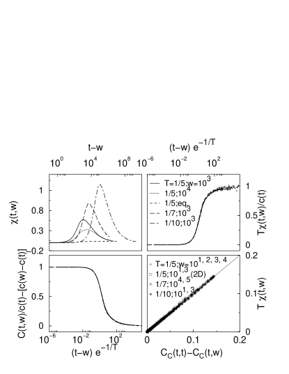
FIG. 1.: Top left: integrated response $\chi(t,w)$ vs. time difference $t-w$ in the 1D FA model. Top right and bottom left: rescaled response Eq. (1) and rescaled autocorrelation function Eq. (2) as a function of scaled time difference $(t-w)e^{-1/T}$. Bottom right: out–of–equilibrium FD relations in the 1D and 2D FA models obtained from parametric plots of response vs. difference of connected autocorrelation.

Having expressed the out–of–equilibrium response and correlation functions in terms of the equilibrium ones, we can now find the FD relations. Since we know that the equilibrium functions satisfy the FD theorem (FDT) [5], $T\chi_{\rm eq}(\tau)=C_{\rm eq}(0)-C_{\rm eq}(\tau)$, from Eqs.(1) and (2) we obtain,

$$T\chi(t,w)\sim C_{c}(t,t)-C_{c}(t,w),$$ (3)

where $C_{c}(t,t^{\prime})\equiv C(t,t^{\prime})-c(t)c(t^{\prime})$ is the connected autocorrelation function [26]. This means that for all low $T$ and $w>1$ there is a unique dynamical FD relation which corresponds to the out–of–equilibrium response and autocorrelation obeying FDT. We illustrate this for various temperatures and waiting times in Fig. 1 (bottom right) for the 1D and 2D models. Notice that this result does not mean that the system is in equilibrium: one–time quantities, like the defect concentration $c(t)$, are orders of magnitude away from their equilibrium values; and, moreover, from the plateau onwards, the system develops a strong nearest–neighbour repulsion, $\langle\delta n_{i}(t)\delta n_{i\pm 1}(t)\rangle\sim-c(t)[c(t)-c_{\rm eq}]$, which is a manifestation of the fact that the dynamics explores mostly local minima, and eventually vanishes in equilibrium. In fact, the response to a uniform field and the autocorrelation of the magnetization are not related by any sensible FD relation.

Let us turn now to the more interesting case of the two–dimensional square–plaquette model, which consists of a system of Ising spins, $\sigma_{i}=\pm 1$ $(i=1,\dots,N)$, in a square lattice, with ferromagnetic interactions between quartets of neighbouring spins in the vertices of the plaquettes of the lattice, $H=-\sum_{ijkl\in\square}\sigma_{i}\sigma_{j}\sigma_{k}\sigma_{l}$. This model is a special case of the eight vertex model [27] with trivial thermodynamical properties, but whose single spin–flip

FIG. 2.: Top left: concentration of defects $c(t)$ as a function of time after the quench to $T$ in the 2D square–plaquette model. Top right: integrated response $\chi(t,w)$ as a function of time difference $t-w$. Bottom left: rescaled form of response for early times, Eq.(4). Bottom right: rescaled response for late times, Eq.(5), vs. rescaled time $c(t)(t-w)e^{-2/T}$.

dynamics is glassy [23, 28]. The model has a dual representation in terms of noninteracting plaquette variables, $b_{i}\equiv\sigma_{i}\sigma_{j}\sigma_{k}\sigma_{l}$. Since reversing any spin corresponds to inverting the four plaquettes to which it belongs, the spin–flip dynamics becomes a constrained dynamics in the plaquette representation [23].

Isolated excitations or defects ($b_{i}=-1$) in the plaquette model are stable, and have to overcome an energy barrier to move. In contrast to the FA model, however, pairs of neighbouring defects can move at no energy cost: a horizontal (vertical) pair can diffuse freely in a vertical (horizontal) direction, while a diagonal pair cannot diffuse but is free to oscillate. These excitations play an important role. An isolated defect moves by creating a diffusing pair, so that $\Delta E=2$. The single activation barrier means that this model also behaves as a strong glass. Fig. 2 (top left) displays the decay of the concentration of defects $c(t)\equiv N^{-1}\sum_{i}\langle n_{i}(t)\rangle$, where $n_{i}\equiv(1-b_{i})/2$, as a function of time after a quench from a random state to low temperatures [24]. As a consequence of the presence of the diffusing pairs the plateau is reached more slowly than in the FA model. The activated regime corresponds to times $t>10^{2}$ and $T<0.25$ in this case. At the plateau the defect concentration is $c_{P}=0.089$, that of moving pairs is $O(e^{-1/T}c_{P})$, and that of defects which belong to oscillating pairs is finite, $d_{P}=0.026$.

In analogy with the FA model, we now consider the linear response of the excitations $n_{i}$, instead of that of the spins $\sigma_{i}$ which in this class of models do not obey any systematic out–of–equilibrium FD relations [17]. In Fig. 2 (top right) we show the integrated response function of individual excitations, $\chi(t,w)$, for $w>10^{2}$ and low temperatures. The response is again non–monotonic, but in this case it also presents an intermediate saturation at early time lag. This is a consequence of the existence of two well separated relevant timescales. The early behaviour is due to the fast response of the oscillating pairs, which exist in finite number in the activated regime. This means that we expect, to leading order in $e^{-1/T}$, the scaling form of the response function for low $T$, $w>10^{2}$, and $t-w\sim O(1)$ to be,

$$T\chi(t,w)\sim d(t)\,f(t-w),$$ (4)

where $d(t)$ is the number of excitations which belong to an oscillating pair as a function of time, and $f(\tau)$ is an increasing, temperature independent, function, which should saturate at a half, $f(\infty)=1/2$, given that each oscillator can be in two states. The collapse under (4) of the response curves for early time lags is given in Fig. 2 (bottom left). After the saturation of the oscillators, the response of the isolated defects takes over, so we expect the response function to be proportional to $c(t)$, and the time lag to scale with the relaxation time, so that for $t-w\gg 1$,

$$T\chi(t,w)\sim\frac{1}{2}\,d(t)+c(t)\,g\left[c(t)\frac{(t-w)}{e^{2/T}}\right],$$ (5)

where $g(\tau)$ is a temperature independent function with $g(\infty)=1$, and the relaxation time $\tau_{rel}\sim e^{2/T}/c(t)$ for the diffusion of isolated defects scales with time through $c(t)$ to account for the necessary number of diffusing pairs created to reach another isolated defect. This rather unexpected behaviour comes from the restricted 1D motion of the diffusing pairs and leads to a relaxation time $\tau_{rel}\sim e^{3/T}$ in equilibrium. In Fig. 2 (bottom right) we show that (5) accurately scales all the response curves for long time lags. Similar scaling relations can be obtained for the autocorrelation function.

The existence of two relevant timescales for the out–of–equilibrium dynamics naturally leads to the question of whether response and correlation obey nontrivial FD relations. In Fig. 3 we present the FD plot obtained para-

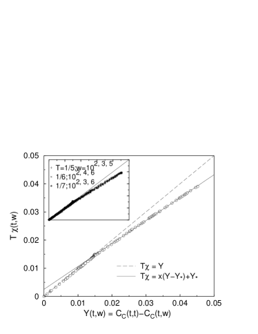
FIG. 3.: Out–of–equilibrium FD relations in the 2D square–plaquette model. The inset gives the FD plots for various $T$ and $w$. The main figure is the average of all the data. The error bars are comparable to the size of the symbols. A linear fit to the second part of the curve gives a slope $x=0.81$ and breaking point $Y_{*}=0.013$.

metrically from the integrated response $\chi(t,w)$ against the difference of the connected autocorrelation $Y(t,w)\equiv C_{c}(t,t)-C_{c}(t,w)$ for different temperatures and waiting times. The remarkable thing is that the FD relations for all the values of $T$ and $w$ fall in a unique master FD plot. The FD curve has the piecewise linear structure characteristic of discontinuous mean–field models [6], with a single breaking point $Y_{*}=0.013$ and slope $x=0.81$.

Several comments are in order. The autocorrelation difference $Y(t,w)$ is playing the role of (one minus) the overlap between configurations in this physical aging situation. The dependence of the response on time is through this difference, $\chi(t,w)=\chi[Y(t,w)]$. Moreover, while $Y(t,w)$ is a non–monotonic function of $t$, it is a monotonic function of $w$, so the FD relation can be rewritten $T\chi(Y)=\int_{0}^{Y}X(y)dy$, where $X(y)=1$ for $y<Y_{*}$, and $X(y)=x$ for $y>Y_{*}$. Notice also that for fixed $t$ and varying $w$, the range of $Y$ is determined by $c(t)$, i.e., $Y(t,w)\in[0,c(t)-c^{2}(t)]$, and given that for all temperatures under consideration $Y_{\rm eq}(\infty)<Y_{*}$, all equilibrium curves are contained in the master plot of Fig. 3.

The piecewise linear FD plot is purely a dynamical effect—the static properties of the model are trivial. This means that violation of FDT does not necessarily entail an RSB–like phase transition as in disordered mean–field models [8]. The configurations at the plateau seem to determine the structure of the FD curve. Each of these is composed of $c_{P}$ excitations, $d_{P}$ of which belong to an oscillating pair. The breaking point $Y_{*}=d_{P}/2$ is given precisely by the oscillation of all of these pairs. Higher values of $Y$ correspond to pairs of configurations mutually accessible only through activation. It is harder to understand the slope $x$. The fact that it is independent of $T$ means that it is not directly related to the entropy of configurations of isolated defects at the plateau, which can be calculated from the hard–square model [27].

The results of this work suggest that nontrivial FD relations may also exist in the activated regime of more realistic strong glasses than the ones studied here, and in the physical aging regime of other systems with simple statics. While this would only be true for an appropriately defined class of observables, consistent with the remarks of [29], for this class FD relations would be well defined and unique. For the simple models considered here it corresponds to observables constructed out of local energy excitations, which are ‘orthogonal’ to the ones responsible for the activated relaxation, the defect concentration in the case of these systems. It would be interesting to understand the FD ratio $X(y)$ in terms of a geometrical, rather than equilibrium, probability distribution for the dynamical configurations, in line with the ideas of ‘Edward’s measures’ put forward in [14]. And it would also be important to extend these results to the more difficult case of fragile systems.

We thank Josef Jäckle and Peter Sollich for discussions. This work was supported by EU Grant No. HPMF-CT-1999-00328 and the Glasstone Fund (Oxford).

REFERENCES

- [1]
- [2] C.A. Angell, Science 267, 1924 (1995).
- [3] J.-P. Bouchaud, L.F. Cugliandolo, J. Kurchan and M. Mézard, in Spin-glasses and random fields, edited by A.P. Young, (World Scientific, Singapore, 1997).
- [4] P.G. Debenedetti and F.H. Stillinger, Nature 410, 259 (2001).
- [5] See, e.g., D. Chandler, Introduction to Modern Statistical Mechanics, (OUP, Oxford, 1987).
- [6] L.F. Cugliandolo and J. Kurchan, Phys. Rev. Lett. 71, 173 (1993).
- [7] L.F. Cugliandolo, J. Kurchan and L. Peliti, Phys. Rev. E 55, 3898 (1997).
- [8] S. Franz, M. Mézard, G. Parisi and L. Peliti, Phys. Rev. Lett. 81, 1758 (1998).
- [9] A. Barrat, Phys. Rev. E 57, 3629 (1998).
- [10] C. Godrèche and J. M. Luck, J. Phys. A 33, 1151 (2000).
- [11] G. Parisi, Phys. Rev. Lett. 79, 3660 (1997).
- [12] J.L. Barrat and W. Kob, Europhys. Lett. 46, 637 (1999).
- [13] F. Ricci–Tersenghi, D.A. Stariolo and J.J. Arenzon, Phys. Rev. Lett. 84, 4473 (2000).
- [14] A. Barrat, J. Kurchan, V. Loreto and M. Sellitto, Phys. Rev. Lett. 85, 5034 (2000).
- [15] L.C.E. Struik, Physical Aging in Amorphous Polymers and Other Materials, (Elsevier, Houston, 1978).
- [16] A. Crisanti, F. Ritort, A. Rocco and M. Sellitto, J. Chem. Phys. 113, 10615 (2001).
- [17] J.P. Garrahan and M.E.J. Newman, Phys. Rev. E 62, 7670 (2000).
- [18] M. Nicodemi, Phys. Rev. Lett. 82, 3734 (1999).
- [19] L. Santen and W. Krauth, Nature 405, 550 (2000).
- [20] G.H. Fredrickson and H.C. Andersen, Phys. Rev. Lett. 53, 1244 (1984).
- [21] M. Schulz and S. Trimper, J. Stat. Phys. 94 173 (1999).
- [22] A. Buhot and J.P. Garrahan, Phys. Rev. E 64, 21505 (2001).
- [23] A. Lipowski, J. Phys. A 30, 7365 (1997); J.P. Garrahan, J. Phys. Condens. Matter 14, 1571 (2002).
- [24] Simulations were performed using continuous time Monte Carlo[25] for – averaged over – runs. The strength of the perturbations, –, was small enough to be in the linear response regime.
- [25] M.E.J. Newman and G.T. Barkema, Monte Carlo Methods in Statistical Physics, (OUP, Oxford, 1999).
- [26] FD relations are in terms of connected correlations due to the fact that one–time quantities change with time. This can be seen by considering a similar perturbation to the one in the text, but restricted to , which leads to the same response, but only their connected correlation functions coincide in the thermodynamic limit. Alternatively, from the fact that FD relations for should be the same as those for .
- [27] R.J. Baxter, Exactly Solved Models in Statistical Mechanics, (Academic Press, London, 1982).
- [28] For a discussion of aging in other four–spin interaction models see e.g., F. Mila and D. Dean, cond-mat/0109406.
- [29] S. Fielding and P. Sollich, Phys. Rev. Lett. 88, 50603 (2002).