Hebbian imprinting and retrieval in oscillatory neural networks

Abstract

We introduce a model of generalized Hebbian learning and retrieval in oscillatory neural networks modeling cortical areas such as hippocampus and olfactory cortex. Recent experiments have shown that synaptic plasticity depends on spike timing, especially on synapses from excitatory pyramidal cells, in hippocampus and in sensory and cerebellar cortex. Here we study how such plasticity can be used to form memories and input representations when the neural dynamics are oscillatory, as is common in the brain (particularly in the hippocampus and olfactory cortex). Learning is assumed to occur in a phase of neural plasticity, in which the network is clamped to external teaching signals. By suitable manipulation of the nonlinearity of the neurons or of the oscillation frequencies during learning, the model can be made, in a retrieval phase, either to categorize new inputs or to map them, in a continuous fashion, onto the space spanned by the imprinted patterns. We identify the first of these possibilities with the function of olfactory cortex and the second with the observed response characteristics of place cells in hippocampus. We investigate both kinds of networks analytically and by computer simulations, and we link the models with experimental findings, exploring, in particular, how the spike timing dependence of the synaptic plasticity constrains the computational function of the network and vice versa.

1 Introduction

It has long been known that the brain is a dynamical system in which non-static activities are common. In particular, oscillatory neural activity has been observed and is believed to play significant functional roles in, for example, the hippocampus and the olfactory cortex. The inputs to these areas can be oscillatory, and the intra-areal connections also make these systems prone to intrinsic oscillatory dynamics. Networks of interacting excitatory and inhibitory neurons (E-I networks) are ubiquitous in the brain, and oscillatory activity is not unexpected in such networks because of the intrinsically asymmetric character of the interactions between excitatory and inhibitory cells. Recent experimental findings further underscored the importance of dynamics by showing that long term changes in synaptic strengths depend on the relative timing of pre- and postsynaptic firing[1, 2, 3, 4, 5]. For instance, in neocortical and hippocampal pyramidal cells [1, 2, 3, 4, 5, 6, 7], the synaptic strength increases (long-term potentiation (LTP)) or decreases (long-term depression (LTD)), depending on whether the presynaptic spike precedes or follows the postsynaptic one. This synaptic modification is largest for differences between pre- and postsynaptic spike times of order 10 ms. Since the scale of this relative timing is comparable to the period of neural oscillations, the oscillatory dynamics should affect the resulting synaptic modifications. In particular, the relative phases between the oscillating neurons ought to constrain the synaptic changes that can occur. These synaptic strengths should, in turn, determine the nature of the network dynamics. This interplay seems likely to have significant functional consequences.

While we have achieved some understanding of the computational power of oscillatory networks (see [8] and references therein), they are poorly-understood in comparison with networks that always converge to static states, such as feed-forward networks or recurrent networks with symmetric connections. In particular, while we know a lot about appropriate learning algorithms for associative memory in symmetrically-connected and feedforward networks [9], there is little previous work on learning, in the context of the synaptic physiological findings mentioned above, in asymmetrically connected networks with oscillatory dynamics. In this paper, we introduce a model for spike-timing dependent learning in an oscillatory neural network and show how such a network can perform associative memory or input representation after learning.

The experimental findings dictate the general form of our model. It is an E-I (excitatory-inhibitory) network, with asymmetric interactions between excitatory and inhibitory cells, that exhibits input-driven oscillatory activity. We describe the long-term synaptic changes induced by a pair of pre- and postsynaptic spikes at times $t_{pre}$ and $t_{post}$ by a function, which we denote $A(\tau)$, of the difference in spike times $\tau=t_{post}-t_{pre}$. Hence, $A(\tau)$ is positive or negative for LTP or LTD for a particular $\tau$ value. According to the experiments [1, 2, 3, 4, 5, 6, 7], $A(\tau)$ varies in different preparations. For instance, the synapses between hippocampal pyramidal cells have $A(\tau)>0$ when $\tau>0$ and $A(\tau)<0$ when $\tau<0$ We will consider a general $A(\tau)$ in order to be able to explore the consequences of different forms of this function which may be relevant to different areas or conditions. We study analytically and by simulation how oscillatory activities influence synaptic changes and how these changes influence the network oscillations and their functions. In particular, we ask the following questions: (1) How can the system function as an associative memory or as a substrate for a map of an input space? (2) What constraints do these functions place on the form of $A(\tau)$? (3) What constraints would particular experimental findings about $A(\tau)$ impose on the function of networks like this one?

In the next section we present the model E-I network and describe its dynamics for arbitrary synaptic strengths, making use of a linearized analysis. Section 3 then applies the spike-timing-dependent synaptic dynamics to the firing states evoked by oscillatory input. We obtain general expressions for the resulting learned synaptic strengths and use the linearized theory to study the response properties of the network. We show how the learning rates can be adjusted so that, after learning, the network responds strongly (resonantly) to inputs similar to those used to drive it during learning and weakly to unlearned inputs. In addition to this pattern tuning, the system exhibits tuning with respect to driving frequency: the response is weakened for driving frequencies different from that used during learning.

We show further that, depending on the kind of nonlinearity in the neuronal input-output function, the model can perform two qualitatively different kinds of computations. One is associative memory, in which an input to the network is categorized by identifying it with the learned pattern most similar to it. (Olfactory cortex is believed to operate in something like this way.) The other is to make a representation of the input pattern as a continuous mapping onto the space spanned by the learned patterns. For this mode of operation, which we call “input representation”, it is not necessary for the network to have learned explicitly all patterns to which it should respond; it performs a kind of interpolation between a much smaller number of prototypes. (In the hippocampus, we identify these prototypes with place cell fields.) Section 4 presents the nonlinear analysis of the network for both these cases. In Section 5 we examine the consequences of various possible constraints on the signs and plasticities of the synapses. Despite the primitive character of the model we use, we believe our findings may have relevance to the dynamics of many cortical areas. In the final section we discuss our results in the context of other modeling and experimental findings, indicating some interesting directions, both experimental and theoretical, for future work.

2 The model

We base our model on one formulated recently by two of us [10] to describe olfactory cortex. For completeness, we summarize its main features here. In the brain regions we model, hippocampus or olfactory cortex, pyramidal cells make long range connections both to other pyramidal cells and to inhibitory interneurons, while inhibitory interneurons generally only project locally (Fig. 1A). The elementary module of the system is an E-I pair consisting of one excitatory and one inhibitory unit, mutually connected. Each such unit represents a local assembly of pyramidal cells or local interneurons sharing common, or at least highly correlated, input. (The number of neurons represented by the excitatory units is in general different from the number represented by the inhibitory units.) Such E-I pairs, without connections between them, form independent damped local oscillators. The connections between units in different pairs, which we term long range connections, are subject to learning or plasticity in this study. They couple the pairs and determine the normal modes of the coupled-oscillator system. The input to the system is an oscillating pattern $I_{i}$ driving the excitatory units. It models the bulb input to the pyramidal cells in the olfactory cortex or the input from the enthorinal cortex (perforant path) and the dentate gyrus (mossy-fiber) to CA3 pyramidal cells. The system outputs are from the excitatory cells.

Figure 1: A: The model elements. Input is to the excitatory units $u$, which also provide the network output. There are local excitatory-inhibitory connections (vertical solid lines) and nonlocal connections (indicated by dashed lines) between the excitatory units ($J_{ij}$) and from excitatory to inhibitory units ($W_{ij}$). B, C, D: the activation functions for model neurons. Class I and class II nonlinearities are shown in B and C respectively. Crosses mark the equilibrium point $(\bar{u},\bar{v})$ of the system (see Sect. 2.1) used in our numerical simulations. The slopes of all activation functions used in these calculations are taken to be 1 at the equilibrium point. E,F,G: an example of kernel shape $A(\tau)$ [11] and the real and imaginary part of its Fourier transform.

The state variables, modeling the membrane potentials, are ${\bf u}=\{u_{1},\ldots,u_{N}\}$ and ${\bf v}=\{v_{1},\ldots,v_{N}\}$ respectively for the excitatory and inhibitory units. (We denote vectors by bold font.) The unit outputs, representing the probabilities of the cells firing (or instantaneous firing rates) are given by $g_{u}(u_{1}),\ldots,g_{u}(u_{N})$ and $g_{v}(v_{1}),\ldots,g_{v}(v_{N})$, where $g_{u}$ and $g_{v}$ are sigmoidal activation functions that model the neuronal input-output relations. The equations of motion are

$$\dot{u}_{i} = -\alpha u_{i}-\beta_{i}^{0}g_{v}(v_{i})+\sum_{j}J_{ij}^{0}g_{u}(u_{j})+I_{i},$$ (1)

$$\dot{v}_{i} = -\alpha v_{i}+\gamma_{i}^{0}g_{u}(u_{i})+\sum_{j\neq i}W_{ij}^{0}g_{u}(u_{j}).$$ (2)

where $\alpha^{-1}$ is the membrane time constant (for simplicity assumed the same for excitatory and inhibitory units), $J_{ij}^{0}$ is the synaptic strength from excitatory unit $j$ to excitatory unit $i$, $W_{ij}^{0}$ is the synaptic strength from excitatory unit $j$ to inhibitory unit $i$, $\beta_{i}^{0}$ and $\gamma_{i}^{0}$ are the local inhibitory and excitatory connections within the E-I pair $i$, and $I_{i}(t)$ is the net input from other parts of the brain. We omit inhibitory connections between pairs here, since the real anatomical long-range connections appear to come predominantly from excitatory cells. (The parameter $\gamma_{i}^{0}$ could be identified as $W_{ii}^{0}$ and the term $\gamma_{i}^{0}g_{u}(u_{i})$ absorbed into the following sum over $j$, but for later convenience, we have written this local term explicitly.) All these parameters are non-negative; the inhibitory character of the second term on the right-hand side of Eqn. (1) is indicated by the minus sign preceding it.

2.1 linearization

The static part $\bar{\bf I}$ of the input determines a fixed point $(\bar{{\bf u}},\bar{{\bf v}})$, given by the solution of equations $\dot{{\bf u}}=0,\dot{{\bf v}}=0$ with ${\bf I}=\bar{\bf I}$. Linearizing the equations (1) and (2) around the fixed point leads to

$$\dot{u_{i}} = -\alpha u_{i}-\beta_{i}v_{i}+\sum_{j}J_{ij}u_{j}+\delta I_{i}$$

$$\dot{v}_{i} = -\alpha v_{i}+\gamma_{i}u_{i}+\sum_{j}W_{ij}u_{j}$$ (3)

where $u_{i}$ and $v_{i}$ are now measured from their fixed point values, $\delta{\bf I}\equiv{\bf I}-\bar{\bf I}\,$, $\beta_{i}=g^{\prime}_{v}(\bar{v}_{i})\beta_{i}^{0}$, $\gamma_{i}=g^{\prime}_{u}(\bar{u}_{i})\gamma_{i}^{0}$, $W_{ij}=g^{\prime}_{u}(\bar{u}_{j})W_{ij}^{0}$ $J_{ij}=g^{\prime}_{u}(\bar{u}_{j})J_{ij}^{0}$. Henceforth, for simplicity, we assume $\beta_{i}=\beta$, $\gamma_{i}=\gamma$, independent of $i$.

Eliminating the $v_{i}$ from (3), we have the second order differential equations

$$\left[(\partial_{t}+\alpha)^{2}+\beta\gamma\right]{\bf u}={\sf M}{\bf u}+(\partial_{t}+\alpha)\delta{\bf I}$$ (4)

$$\mbox{where}\qquad{\sf M}=(\partial_{t}+\alpha){\sf J}-\beta{\sf W}\,,$$ (5)

or, equivalently,

$$\ddot{{\bf u}}+(2\alpha-{\sf J})\dot{{\bf u}}+[\alpha^{2}-\alpha{\sf J}+\beta(\gamma+{\sf W})]{\bf u}=(\partial_{t}+\alpha)\delta{\bf I}.$$ (6)

(We use sans serif to denote matrices.)

Given a stable fixed point, an oscillatory drive $\delta{\bf I}\equiv\delta{\bf I}^{+}+\delta{\bf I}^{-},$ where $\delta{\bf I}^{+}\propto e^{-{\rm i}\omega t}$ and $\delta{\bf I}^{-}=\delta{\bf I}^{+*}$, will lead eventually to a sustained oscillatory response ${\bf u}\equiv{\bf u}^{+}+{\bf u}^{-}$ with the same frequency $\omega$, with ${\bf u}^{+}\propto{\rm e}^{-{\rm i}\omega t}$ and ${\bf u}^{-}={\bf u}^{+*}$. Then from Eqn. (4),

$$\left[(-{\rm i}\omega+\alpha)^{2}+\beta\gamma\right]u_{i}^{+}=\sum_{j}M_{ij}u_{j}^{+}+\left(\alpha-{\rm i}\omega\right)\delta I_{i}^{+},$$ (7)

where

$${\sf M}=(\alpha-{\rm i}\omega){\sf J}-\beta{\sf W}.$$ (8)

is now the ${\sf M}$ in equation (5) applied to the $e^{-{\rm i}\omega t}$ modes. The terms in the square bracket describe the local E-I pair contribution, while ${\sf M}$ gives an effective coupling between the oscillating E-I pairs. A zero ${\sf M}$ makes ${{\bf u}}$ proportional to $\delta{\bf I}$ with a constant phase shift, i.e., each individual damping oscillator is driven independently by a component of the external drive. Learning imprints patterns into ${\sf M}$ through the long range connections $\sf J$ and $\sf W$. After learning, ${{\bf u}}$ depends on how $\delta{\bf I}^{+}$ decomposes into the eigenvectors of ${\sf M}$. Thus the network can selectively amplify or distort $\delta{\bf I}$ in an imprinted-pattern-specific manner and thereby function as an associative memory or input representation.

2.2 Nonlinearity

At large response amplitudes, nonlinearity in $g_{u}$ and $g_{v}$ significantly modifies the response. We will focus on the nonlinearity in $g_{u}$ only, since $g_{v}$ only affects the local synaptic input while $g_{u}$ also affects the long range input mediated by $\sf J$ and $\sf W$. We categorize the nonlinearity into 2 general classes in terms of how $g_{u}$ deviates from linearity near the fixed point $\bar{\bf u}$:

$$\mbox{class I:}~{}~{}~{}~{}~{}~{}g_{u}(u_{i})\sim u_{i}-au_{i}^{3}~{}~{}~{}~{}~{}~{}~{}~{}~{}~{}\mbox{class II:}~{}~{}~{}~{}~{}~{}g_{u}(u_{i})\sim u_{i}+au_{i}^{3}-bu_{i}^{5}$$ (9)

where $a,b>0$, and $u_{i}$ is measured from the fixed point value $\bar{u}_{i}$. Class I and II nonlinearity differ in whether the gain $g^{\prime}_{u}$ decreases or increases (before saturation) as one moves away from the equilibrium point, and will lead to qualitatively different behavior, as will be shown. We will not treat the more general case where $g_{u}(u)$ is not an odd function of $u$. However, to lowest order a quadratic term just acts to shift the equilibrium point, and a quartic one does not affect our results qualitatively.

3 Learning, neural dynamics, and model behavior

In our treatment, we distinguish a learning mode, in which the oscillating patterns are imprinted in the synaptic connections $\sf J$ and $\sf W$, from a recall mode, in which connection strengths do not change. Of course, this distinction is somewhat artificial; real neural dynamics may not be separated so cleanly into such distinct modes. Nevertheless, cholinergic modulatory effects probably do weaken synapses during learning [12], so there is an experimental basis for the distinction, and it is conceptually indispensable.

In what follows we will consider learning of oscillation patterns of two kinds. In one, two local oscillators are either in phase with each other or $180^{\circ}$ out of phase, i.e., we can write $u_{i}(t)\propto\xi_{i}\cos\omega t$, where the $\xi_{i}$ are real numbers (either positive or negative) describing the amplitudes on the different sites. In the second kind of pattern, different local oscillators can have different phases: $u_{i}(t)\propto|\xi_{i}|\cos(\omega t-\phi_{i})$. We can describe both cases by writing $u_{i}(t)=\xi_{i}{\rm e}^{-{\rm i}\omega t}+{\rm c.c.}$, taking the $\xi_{i}$ real in the first case and complex ($\xi_{i}=|\xi_{i}|{\rm e}^{{\rm i}\phi_{i}}$) in the second. Thus we will often call the first case “real patterns” and the second “complex patterns”.

3.1 learning mode

Let $C_{ij}$ be the synaptic strength from presynaptic unit $j$ to postsynaptic unit $i$. Let $x_{j}(t)$ and $y_{i}(t)$ represent the corresponding activities relative to some stationary levels at which no changes in synaptic strength occur. Then $C_{ij}$ changes during the learning interval $[0,T]$ according to

$$\delta C_{ij}(t)=\langle y_{i}(t)A(t-t^{\prime})x_{j}(t^{\prime})\rangle=\frac{\eta}{T}\int_{0}^{T}{\rm d}t\int_{-\infty}^{\infty}{\rm d}t^{\prime}\,y_{i}(t)A(t-t^{\prime})x_{j}(t^{\prime}).$$ (10)

where $\eta$ is the learning rate and $T$ may be taken equal to the period of the oscillating input. The kernel $A(t-t^{\prime})$ is the measure of the strength of synaptic change at time delay $\tau=t-t^{\prime}$. For example, conventional Hebbian learning, with $A(\tau)\propto\delta(\tau)$ (used, e.g., in [10]), gives $\delta C_{ij}\propto\int_{0}^{T}{\rm d}t\,u_{i}(t)u_{j}(t)$. Some experiments [3, 4] suggest $A(\tau)$ to be a nearly antisymmetric function of $\tau$, positive (LTP) for $\tau>0$ and negative (LTD) for $\tau<0$ (see Fig. 1EFG). However, for the moment we do not restrict its shape.

Applying the learning rule to our connections $J_{ij}$ and $W_{ij}$, we use Eqn. (10) with ${\bf x}={\bf u}$, ${\sf C}={\sf J}$ or $\sf W$, and ${\bf y}={\bf u}$ or $\bf v$, respectively, giving:

$$J_{ij} = \frac{1}{NT}\int_{0}^{T}{\rm d}t\int_{-\infty}^{\infty}{\rm d}t^{\prime}\,u_{i}(t)A_{J}(t-t^{\prime})u_{j}(t^{\prime})$$

$$W_{ij} = \frac{1}{NT}\int_{0}^{T}{\rm d}t\int_{-\infty}^{\infty}{\rm d}t^{\prime}\,v_{i}(t)A_{W}(t-t^{\prime})u_{j}(t^{\prime}).$$ (11)

We have absorbed the learning rates into the definition of the kernels $A_{J,W}$ and added the conventional normalizing factor $1/N$ for convenience in doing the mean field calculations.

As mentioned above, cholinergic modulation can affect the strengths of long-range connections in the brain; these are apparently almost ineffective during learning [12]. The neural dynamics is then simplified in our model by turning off $\sf J$ and $\sf W$ (and thus ${\sf M}$) in the learning phase.

Consider the learning of a single input pattern, $\delta{\bf I}=\boldsymbol{\xi}^{\mu}e^{-{\rm i}\omega_{\mu}t}+{\rm c.c.}$. We calculate separately the responses $u_{i}^{\pm}$ and $v_{i}^{\pm}$ to the positive- and negative-frequency parts of the input, add them together, and use the resulting $u_{i}(t)$ and $v_{i}(t)$ in Eqns. (11) to calculate $J_{ij}$ and $W_{ij}$. For the positive-frequency response we obtain

$$u_{i}^{+} = \frac{(\alpha-{\rm i}\omega_{\mu})\xi_{i}^{\mu}{\rm e}^{-{\rm i}\omega_{\mu}t}}{(\alpha-{\rm i}\omega_{\mu})^{2}+\beta\gamma}\equiv\chi_{0}(\omega_{\mu})\xi_{i}^{\mu}{\rm e}^{-{\rm i}\omega_{\mu}t}$$ (12)

$$v_{i}^{+} = \frac{\gamma}{\alpha-{\rm i}\omega_{\mu}}\chi_{0}(\omega_{\mu})\xi_{i}^{\mu}{\rm e}^{-{\rm i}\omega_{\mu}t}.$$ (13)

The quantity $\chi_{0}(\omega)$ is the output-to-input ratio for the network with $\sf J$ and $\sf W$ equal to zero. The responses $u_{i}^{-}$ and $v_{i}^{-}$ to the corresponding negative-frequency driving pattern $\delta{\bf I}^{-}=\boldsymbol{\xi}^{\mu*}e^{{\rm i}\omega_{\mu}t}$ are the complex conjugates of (12) and (13), respectively.

Substituting these responses into Eqns. (11) yields connections

$$J_{ij}^{\mu} = \frac{2}{N}{\rm Re}\,[\tilde{A}_{J}({\omega_{\mu}})\,\xi_{i}^{\mu}\xi_{j}^{\mu*}]$$

$$W_{ij}^{\mu} = \frac{2\gamma}{N}{\rm Re}\,\big{[}\frac{\tilde{A_{W}}({\omega_{\mu}})}{\alpha-{\rm i}\omega_{\mu}}\xi_{i}^{\mu}\xi_{j}^{\mu*}\big{]},$$ (14)

where

$$\tilde{A}_{J,W}(\omega)=|\chi_{0}(\omega)|^{2}\int_{-\infty}^{\infty}{\rm d}\tau\,A_{J,W}(\tau){\rm e}^{-{\rm i}\omega\tau}$$ (15)

can be thought of as an effective learning rate at a frequency $\omega$. The factor of the Fourier transform of the learning kernel carries the information about different efficacies of learning for different postsynaptic-presynaptic spike time differences, while the factor $|\chi_{0}(\omega)|^{2}$ reflects the responsiveness of the uncoupled local oscillators (${\sf J}={\sf W}=0$) in the learning phase. Note that ${\rm Im}\,\tilde{A}_{J,W}(\omega)=0$ if $A_{J,W}(\tau)$ is symmetric in $\tau$ and that ${\rm Re}\,\tilde{A}_{J,W}(\omega)=0$ if $A_{J,W}(\tau)$ is antisymmetric. We will sometimes denote the real and imaginary parts of $\tilde{A}_{J,W}$ by $\tilde{A}^{\prime}_{J,W}$ and $\tilde{A}^{\prime\prime}_{J,W}$, respectively.

The resulting effective coupling ${\sf M}$ between oscillators after learning, under positive-frequency external drive $\delta{\bf I}^{+}$ of frequency $\omega>0$ (in general $\omega\neq\omega_{\mu}$), is

$$M_{ij}^{\mu}=\frac{2(\alpha-{\rm i}\omega)}{N}{\rm Re}\,[\tilde{A}_{J}({\omega_{\mu}})\xi_{i}^{\mu}\xi_{j}^{\mu*}]-\frac{2\beta\gamma}{N}\,{\rm Re}\,\big{[}\frac{\tilde{A}_{W}(\omega_{\mu})}{\alpha-{\rm i}\omega_{\mu}}\xi_{i}^{\mu}\xi_{j}^{\mu*}\big{]}$$ (16)

The dependence of the neural connections ${\sf J}$ and ${\sf W}$ and the oscillator couplings ${\sf M}$ on $\xi_{i}^{\mu}\xi_{j}^{\mu*}$ is just a natural generalization of the Hebb-Hopfield factor $\xi_{i}^{\mu}\xi_{j}^{\mu}$ for (real) static patterns. This becomes particularly clear if we consider the special case when there is the following matching condition between the two kernels:

$$\tilde{A}_{J}(\omega_{\mu})=\frac{\beta\gamma}{\alpha^{2}+\omega_{\mu}^{2}}\tilde{A}_{W}(\omega_{\mu}),~{}~{}~{}~{}~{}~{}~{}\omega=\omega_{\mu}.$$ (17)

Then the oscillator coupling simplifies into a familiar outer-product form for complex vectors $\boldsymbol{\xi}$:

$$M_{ij}^{\mu}=-2{\rm i}\omega_{\mu}\tilde{A}_{J}(\omega_{\mu})\xi_{i}^{\mu}\xi_{j}^{\mu*}/N,$$ (18)

To construct the corresponding matrices for multiple patterns (which we will always take to be random and independent) we simply sum (14) over input patterns, labeled by the index $\mu$, as for the Hopfield model. We restrict attention to the case where the number $P$ of stored patterns is negligible in comparison with $N$, the size of the network (though it may be $\gg 1$). So far, all our results apply for both real and complex patterns.

3.2 Recall mode

After learning, the connections are fixed and the response ${\bf u}^{+}$ to an input $\delta{\bf I}^{+}\propto{\rm e}^{-{\rm i}\omega t}$ is described by Eqn. (7). To solve it, we need to know how the ${\sf M}$ matrix acts on input vectors. We consider uncorrelated patterns all learned at the same frequency ($\omega_{\mu}$ independent of $\mu$). Then it is easy to see that ${\sf M}$ is a projector onto the space spanned by the imprinted patterns. It has $P$ eigenvectors (the imprinted patterns) with the same nonzero eigenvalue and $N-P$ with eigenvalue zero. These are standard properties of outer-product constructions for orthogonal vectors; we can treat our $\boldsymbol{\xi}^{\mu}$ as effectively orthogonal here because we are taking the components $\xi_{i}^{\mu}$ to be independent and $N\gg P$ [13].

The nonvanishing eigenvalue of ${\sf M}$, which we denote $\Pi(\omega,\omega_{\mu})$, is simply computed as

$$\Pi(\omega;\omega_{\mu})=(\alpha-{\rm i}\omega)\tilde{A}_{\rm J}(\omega_{\mu})-\frac{\beta\gamma\tilde{A}_{\rm W}(\omega_{\mu})}{\alpha-{\rm i}\omega_{\mu}},$$ (19)

for complex patterns, and

$$\Pi(\omega;\omega_{\mu})=2(\alpha-{\rm i}\omega){\rm Re}\,\tilde{A}_{\rm J}(\omega_{\mu})-2\beta\gamma{\rm Re}\,\big{[}\frac{\tilde{A}_{\rm W}(\omega_{\mu})}{\alpha-{\rm i}\omega_{\mu}}\big{]}$$ (20)

for real patterns.

Thus, from Eqn. (7), the response ${\bf u}^{+}$ to an input $\delta{\bf I}^{+}$ in the imprinted-pattern subspace is

$${\bf u}^{+}=\chi(\omega;\omega_{\mu})\delta{\bf I}^{+},$$ (21)

with the linear response coefficient or susceptibility

$$\chi(\omega;\omega_{\mu})=\frac{\alpha-{\rm i}\omega}{\alpha^{2}+\beta\gamma-\omega^{2}-2{\rm i}\omega\alpha-\Pi(\omega;\omega_{\mu})}.$$ (22)

To achieve a resonant response to an input at the imprinting frequency ($\omega=\omega_{\mu}$), the learning kernels should be adjusted so that both the real and imaginary parts of the denominator in $\chi(\omega_{\mu};\omega_{\mu})$ are close to zero, i.e.,

$$\epsilon \equiv \alpha^{2}+\beta\gamma-\omega^{2}_{\mu}-{\rm Re}\,\Pi(\omega_{\mu};\omega_{\mu})\rightarrow 0,$$ (23)

$$\Delta \equiv 2\omega_{\mu}\alpha+{\rm Im}\,\Pi(\omega_{\mu};\omega_{\mu})\rightarrow 0.$$ (24)

For real patterns, ${\rm Im}\,\Pi(\omega_{\mu};\omega_{\mu})=-2\omega_{\mu}\tilde{A}_{J}^{\prime}$, so $\Delta=2\omega_{\mu}(\alpha-\tilde{A}_{J}^{\prime})$. Thus small $\Delta$ requires a positive $\tilde{A}^{\prime}_{J}>0$, i.e., stronger positive-$\tau$ LTP than negative-$\tau$ LTD for excitatory-excitatory couplings (again, provided the typical values of $\tau$ for which $A_{J}(\tau)$ is sizeable are small compared to the oscillation period). ¿From Eqn. (24),

$$\epsilon=\alpha^{2}+\beta\gamma-\omega^{2}_{\mu}-2{\rm Re}\,\left[\alpha\tilde{A}_{J}(\omega_{\mu})-\frac{\beta\gamma\tilde{A}_{W}(\omega_{\mu})}{\alpha-{\rm i}\omega_{\mu}}\right]$$ (25)

Thus, for a given $\omega_{\mu}$, the resonance condition enforces a constraint on a linear combination of $\tilde{A}_{J}^{\prime}$, $\tilde{A}_{W}^{\prime}$ and $\tilde{A}_{W}^{\prime\prime}$. However, we note that $\tilde{A}_{J}^{\prime\prime}$ does not appear anywhere; it is simply irrelevant to learning real patterns.

For complex patterns,

$$\epsilon = \alpha^{2}+\beta\gamma-\omega^{2}_{\mu}-(\alpha\tilde{A}^{\prime}_{J}+\omega_{\mu}\tilde{A}^{\prime\prime}_{J})+{\frac{\beta\gamma}{\alpha^{2}+\omega_{\mu}^{2}}}(\alpha\tilde{A}^{\prime}_{W}-\omega_{\mu}\tilde{A}^{\prime\prime}_{W})$$ (26)

$$\Delta = 2\omega_{\mu}\alpha+(\alpha\tilde{A}^{\prime\prime}_{J}-\omega_{\mu}\tilde{A}^{\prime}_{J})-{\frac{\beta\gamma}{\alpha^{2}+\omega_{\mu}^{2}}}(\alpha\tilde{A}^{\prime\prime}_{W}+\omega_{\mu}\tilde{A}^{\prime}_{W})$$ (27)

(We have temporarily suppressed the $\omega_{\mu}$-dependence of $\tilde{A}_{J,W}^{\prime}$ and $\tilde{A}_{J,W}^{\prime\prime}$ to save space.) One can get some insight here by considering the time-shifted learning kernels $A_{J}(\tau+\theta_{\mu}/\omega_{\mu})$ and $A_{W}(\tau-\theta_{\mu}/\omega_{\mu})$, where $\theta_{\mu}=\tan^{-1}(\alpha/\omega_{\mu})$. (For $\alpha\sim\omega_{\mu}\approx 40$ Hz, these shifts are around 3 ms.) In terms of the associated frequency-domain quantities,

$$\tilde{B}_{J,W}(\omega)=|\chi_{0}(\omega)|^{2}\int_{-\infty}^{\infty}{\rm d}\tau\,A_{J,W}(\tau\pm\theta_{\mu}/\omega_{\mu}){\rm e}^{-{\rm i}\omega\tau}=\tilde{A}_{J,W}(\omega){\rm e}^{\pm{\rm i}\theta_{\mu}},$$ (28)

we can write Eqns. (26) and (27) as

$$\epsilon = \alpha^{2}+\beta\gamma-\omega^{2}_{\mu}-\sqrt{\alpha^{2}+\omega_{\mu}^{2}}\tilde{B}_{J}^{\prime\prime}(\omega_{\mu})-\frac{\beta\gamma}{\sqrt{\alpha^{2}+\omega_{\mu}^{2}}}\tilde{B}_{W}^{\prime\prime}(\omega_{\mu})$$ (29)

$$\Delta = 2\omega_{\mu}\alpha-\sqrt{\alpha^{2}+\omega_{\mu}^{2}}\tilde{B}_{J}^{\prime}(\omega_{\mu})-\frac{\beta\gamma}{\sqrt{\alpha^{2}+\omega_{\mu}^{2}}}\tilde{B}_{W}^{\prime}(\omega_{\mu}).$$ (30)

Thus, the imaginary parts of the frequency-domain kernels $\tilde{B}_{J,W}(\omega_{\mu})$ shift the resonant frequency and the real parts control the damping. In particular, one needs at least one of $\tilde{B}^{\prime}_{J,W}$ to be positive to achieve good frequency tuning. Negative (positive) imaginary parts $\tilde{B}^{\prime\prime}_{J,W}$ increase (decrease) the resonant frequency.

When the learning window widths in the kernels $A_{J,W}(\tau)$ are much smaller than the oscillation period, the shifts by $\pm\theta_{\mu}/\omega_{\mu}$ do not affect the real parts of $B_{J,W}$ strongly. However, for window shapes (see Fig. 1E) that change rapidly from negative to positive around $\tau=0$, the imaginary parts can be strongly suppressed, even for fairly small shifts.

The explicit form of the resonant response can be seen by expanding the denominator of $\chi(\omega;\omega_{\mu})$ around $\omega=\omega_{\mu}$:

$$\chi(\omega;\omega_{\mu})=\frac{\alpha-{\rm i}\omega_{\mu}}{\epsilon-i\Delta-Z(\omega_{\mu})(\omega-\omega_{\mu})},$$ (31)

where

$$Z(\omega_{\mu})=2\omega_{\mu}+2{\rm i}\alpha+\left.\frac{\partial\Pi(\omega;\omega_{\mu})}{\partial\omega}\right|_{\omega=\omega_{\mu}}.$$ (32)

Thus $\chi$ has a pole at

$$\omega=\omega_{\mu}+\frac{\epsilon-{\rm i}\Delta}{Z}=\omega_{\mu}+\frac{\epsilon Z^{\prime}-\Delta Z^{\prime\prime}-{\rm i}(\Delta Z^{\prime}+\epsilon Z^{\prime\prime})}{|Z|^{2}},$$ (33)

and, as the driving frequency $\omega$ in the recall phase is varied, the system exhibits a resonant tuning, with a peak near $\omega_{\mu}$ and a linewidth equal to $(\Delta Z^{\prime}+\epsilon Z^{\prime\prime})/|Z|^{2}$.

One has to check that the desired learning rates and kernels do not violate the condition that the response function (22) be causal, i.e., small perturbations decay in time. Analytically, the requirement is that all singularities of $\chi(\omega,\omega_{\mu})$ must lie in the lower half of the complex $\omega$ plane. Thus, in Eqn. (33), we need $\Delta Z^{\prime}+\epsilon Z^{\prime\prime}$ to be positive.

For real patterns, the analysis is fairly simple. From Eqns. (20) (24) and (32), we obtain $Z=2\omega_{\mu}+2{\rm i}(\alpha-\tilde{A}_{J}^{\prime})$ and $\Delta=2\omega_{\mu}(\alpha-\tilde{A}_{J}^{\prime})$. Thus, for $\Delta\rightarrow 0$, $Z\rightarrow 2\omega_{\mu}$, and the stability condition is simply that $\Delta$ be positive, i.e., $\tilde{A}_{J}^{\prime}(\omega_{\mu})<\alpha$.

For complex patterns, we get $Z=2\omega_{\mu}+\tilde{A}_{J}^{\prime\prime}+{\rm i}(2\alpha-\tilde{A}_{J}^{\prime})$. Requiring $\Delta Z^{\prime}+\epsilon Z^{\prime\prime}$ to be positive then imposes constraints on the signs and relative magnitudes of $\epsilon$ and $\Delta$, depending on $Z^{\prime}$ and $Z^{\prime\prime}$. We omit the details.

Notice that, for both the real and complex cases, the stability analysis does not depend on the $\sf W$-learning kernel $A_{W}$ at all (except insofar as it affects $\epsilon$ and $\Delta$). This is because $Z$ involves the derivative $\partial\Pi(\omega,\omega_{\mu})/\partial\omega$, and in both cases the only $\omega$-dependence of $\Pi$ is in the factors $(\alpha-{\rm i}\omega)$ in the first terms of Eqns. (19) and (20), which do not involve $\tilde{A}_{W}$.

A

$\omega=\omega_{\mu}$= 33 Hz	$\omega=$ 38 Hz	$\omega=$ 41 Hz	$\omega=$ 49 Hz

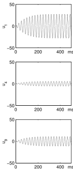
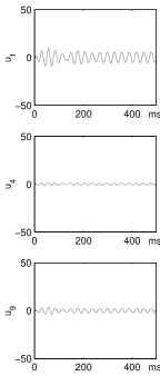
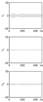
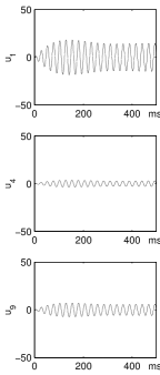
B.1	B.2

Figure 2: Frequency tuning, shown as response to $\delta{\bf I}^{+}=\boldsymbol{\xi}_{\mu}{\rm e}^{-{\rm i}\omega t}$ after imprinting $\boldsymbol{\xi}_{\mu}{\rm e}^{-{\rm i}\omega_{\mu}t}$ with $\omega_{\mu}=$ 41 Hz. The network has 10 excitatory and 10 inhibitory units. In all figures of this paper except where explicitly stated, learning kernels are matched so that $\tilde{A}_{\rm J}=\frac{\beta\gamma}{\alpha^{2}+\omega_{\mu}^{2}}\tilde{A}_{\rm W}=0.5-{\rm i}\,0.028$, and $\omega_{\mu}\sim$ 41 Hz. A: temporal activities of 3 of the 10 excitatory cells. $g_{u}$ and $g_{v}$ are as in Fig. 1BD.  B: frequency tuning curve. Response amplitude $|\langle{\bf u}^{+}|\boldsymbol{\xi}^{\mu}{\rm e}^{-{\rm i}\omega t}\rangle|$ (simply $|\chi(\omega;\omega_{{\mu}})|$ in the linearized theory) to input $\delta{\bf I}^{+}=\boldsymbol{\xi}^{\mu}{\rm e}^{-{\rm i}\omega t}$. B.1: using matched kernel, from linearized theory (solid line) and from class I (stars) and II (circles) nonlinearities. B.2: Opposite-plasticities case ($\tilde{A}_{\rm J}=-\tilde{A}_{\rm W}=0.99(\alpha-{\rm i}\omega_{\mu})$), complex patterns. Dashed line, circles, and triangles are results from the linearized theory and the class II nonlinear model with $\omega_{\mu}=41Hz$ and $\omega_{\mu}=68Hz$ respectively.

Fig. 2 shows examples of the frequency tuning described by Eqn. (31), as obtained from simulations of small networks, including the nonlinearities described in Sect. 2.2. Nonlinearity makes the response deviate from the linear prediction when the amplitude is larger, as happens near the resonance frequency. In particular, class I and class II nonlinearities lead to reduced and enhanced responses, respectively relative to the linear prediction, as will be analyzed in detail later.

3.2.1 Examples of plasticity

We use examples to illustrate the constraints that resonance and stability conditions place on the shape of the kernels for complex patterns.

$\sf J$ only

If the patterns are imprinted only in the excitatory-excitatory connections, we have only the first terms on the right-hand sides of Eqns. (19) and (20).

For real patterns $\Delta=2\omega_{\mu}(\alpha-\tilde{A}_{J}^{\prime})$ (no different from the general case), so, using $\Delta\rightarrow 0$ in Eqn. (25) yields $\epsilon=\beta\gamma-\alpha^{2}-\omega^{2}_{\mu}$. This then (from $\epsilon=0$) fixes the imprinting frequency $\omega_{\mu}=\sqrt{\beta\gamma-\alpha^{2}}$.

For complex patterns, we have $\Delta=2\omega_{\mu}\alpha-\sqrt{\alpha^{2}+\omega_{\mu}^{2}}\tilde{B}_{J}^{\prime}$, i.e., similar to the real-pattern case but with a shifted learning window and a different effective strength. The resonant frequency shifts down or up according to the sign of $\tilde{B}_{J}^{\prime\prime}$.

Same-sign plasticities in ${\sf J}$ and ${\sf W}$

Let us consider the case where the kernels are related by the matching condition (17). While the exact match is clearly a special case, the simplification it yields in the algebra permits some insight which can be expected to carry over qualitatively to other cases where the two kernels have similar shapes and comparable magnitudes. Here we find, from Eqns. (19) and (20),

$$\Pi(\omega_{\mu};\omega_{\mu})=-2{\rm i}\omega_{\mu}\tilde{A}_{J}(\omega_{\mu}),$$ (34)

for both real and complex patterns. Applying the resonance condition equations (23, 24), we have

$$\tilde{A}_{J}^{\prime\prime}(\omega_{\mu}) = \frac{-\omega_{\mu}^{2}+\alpha^{2}+\beta\gamma-\epsilon}{2\omega_{\mu}}$$ (35)

$$\tilde{A}_{J}^{\prime}(\omega_{\mu}) = \alpha-\Delta/2\omega_{\mu}$$ (36)

Thus $\tilde{A}_{J}^{\prime}(\omega_{\mu})$ reduces the effective damping from $\alpha$ to $\Delta/2\omega_{\mu}\ll\alpha$, and this requires $\tilde{A}^{\prime}(\omega_{\mu})\approx\alpha>0$. When the width of the learning kernel $A_{J}(\tau)$ is much smaller than the oscillation period, $\tilde{A}_{J}^{\prime}(\omega_{\mu})\approx\int A_{J}(\tau){\rm d}\tau$, thus a positive $\tilde{A}_{J}^{\prime}(\omega_{\mu})$ requires that LTP dominate LTD in total strength.

We observe that a negative $\tilde{A}_{J}^{\prime\prime}(\omega_{\mu})$, i.e., an $A_{J}(\tau)$ like that in Fig. 1EFG, forces $\omega_{\mu}$ to be greater than $\sqrt{\alpha^{2}+\beta\gamma}$ and thus greater than the intrinsic E-I pair frequency $\sqrt{\beta\gamma}$ (a shift in the opposite direction from that in the $\sf J$-only, real-pattern case).

In general, when the width of $A_{J}(\tau)$ is not small, the resonance frequency has to be determined from equations (35) and (36) by $\tilde{A}_{J}^{\prime\prime}(\omega_{\mu})/\tilde{A}_{J}^{\prime}(\omega_{\mu})\approx(-\omega_{\mu}^{2}+\alpha^{2}+\beta\gamma)/2\alpha\omega_{\mu}$.

Opposite-sign plasticities in ${\sf J}$ and ${\sf W}$

We turn now to the case where $A_{J}(\tau)$ and $A_{W}(\tau)$ have opposite signs (for all $\tau$). Again, we turn to a particular matching of the magnitudes of the two kernels to find a simple case that can give some general qualitative insight. We use our old matching condition, Eqn. (17), but with a minus sign. For complex patterns we now find $\Pi(\omega_{\mu},\omega_{\mu})=2\alpha\tilde{A}_{J}(\omega_{\mu})$, and, applying the resonance condition equations (23, 24),

$$\tilde{A}_{J}^{\prime}(\omega_{\mu}) = \frac{-\omega_{\mu}^{2}+\alpha^{2}+\beta\gamma-\epsilon}{2\alpha}$$ (37)

$$-\tilde{A}_{J}^{\prime\prime}(\omega_{\mu}) = \omega_{\mu}-\Delta/2\alpha$$ (38)

Comparing these with equations (35) and (36) and the accompanying analysis, we see that the roles of the real and imaginary parts of $\tilde{A}_{J}$ have been reversed: Now it is the imaginary part that is constrained to be near a fixed value ($-\omega_{\mu}$) by the $\Delta\rightarrow 0$ condition, and the real part that enters in the $\epsilon$ equation. We note that we need $\tilde{A}_{J}^{\prime\prime}(\omega_{\mu})<0$ (i.e. like the case shown in Fig. 1E), in order to obtain a small $\Delta$, and that the sign of $\tilde{A}^{\prime}(\omega_{\mu})$ determines whether the the resonance frequency is larger or smaller than $\sqrt{\alpha^{2}+\beta\gamma}$.

Another interesting special case for complex patterns is when $A_{W}=-A_{J}$, with the particular choice

$$\tilde{A}_{J}(\omega_{\mu})=\alpha-{\rm i}\omega_{\mu}$$ (39)

This leads to the remarkably simple result

$$\chi(\omega;\omega_{\mu})=\frac{{\rm i}}{\omega-\omega_{\mu}}.$$ (40)

That is, the choice (39) satisfies both constraints, $\epsilon,\Delta\rightarrow 0$ and, in addition, puts the resonance right at the original driving frequency. Fig. 2.B.2 shows a frequency tuning curve obtained with $\tilde{A}_{J}(\omega_{\mu})=0.99(\alpha-{\rm i}\omega_{\mu})$.

To understand the prescription $\tilde{A}_{J}(\omega_{\mu})=\alpha-{\rm i}\omega_{\mu}$, consider an oscillation period much greater than the temporal width of the learning kernel. Then $\tilde{A}_{J}^{\prime}(\omega_{\mu})\approx\int A(\tau)d\tau$ and $\tilde{A}^{\prime\prime}(\omega_{\mu})\approx-\int A_{J}(\tau)\omega_{\mu}\tau d\tau\propto-\omega_{\mu}$. Thus the prescription just requires $\int A_{J}(\tau)d\tau\approx\alpha>0$ (LTP dominates LTD in total strength) and $\int A_{J}(\tau)\tau d\tau\approx 1>0$ (LTP when postsynaptic spikes follow presynaptic ones, and LTD for the opposite order). This means that $A_{J}(\tau)$ should look like Fig. 1E and $A_{W}(\tau)$ like its negative.

We remark that for real patterns this choice of kernels does not produce resonant oscillations; in fact, it leads to instability.

3.2.2 Pattern selectivity

We now consider an input $\delta{\bf I}^{+}{=\boldsymbol{\xi}{\rm e}^{-{\rm i}\omega t}}$ that does not match the imprinted pattern $\boldsymbol{\xi}^{\mu}$. In general, we can decompose it into a component along $\boldsymbol{\xi}^{\mu}$ and a component in the complementary subspace: $\delta{\bf I}^{+}\equiv\delta{\bf I}^{+}_{\|}+\delta{\bf I}^{+}_{\perp}$, with $\delta{\bf I}^{+}_{{\|}}\equiv\langle\boldsymbol{\xi}^{\mu}|\boldsymbol{\xi}\rangle\boldsymbol{\xi}^{\mu}{\rm e}^{-{\rm i}\omega t}\equiv N^{-1}(\sum_{j}\xi_{j}^{\mu*}\xi_{j})\boldsymbol{\xi}^{\mu}{\rm e}^{-{\rm i}\omega t}$. then, ${\sf M}{\bf I}^{+}=\Pi(\omega;\omega_{\mu}){\bf I}^{+}_{{\|}}$, and

$${\bf u}^{+}=\chi(\omega;\omega_{\mu})\delta{\bf I}^{+}_{{\|}}+\chi_{0}(\omega)\delta{\bf I}^{+}_{\perp}.$$ (41)

The first term will be resonant at $\omega=\omega_{\mu}$, but the second will not. Thus, the system amplifies the component of the input along the stored pattern relative to the orthogonal one, as shown in Fig. 3. Again, nonlinearity makes the response deviate from the linear prediction at high response amplitudes, reducing and enhancing the responses for the class I and II nonlinearities, respectively. Class II nonlinearity also leads to hysteresis, with sustained responses even after the input is withdrawn, i.e., $|\langle{\boldsymbol{\xi}^{{\mu}}}|\boldsymbol{\xi}\rangle|\rightarrow 0$. The pattern selectivity can be measured by the ratio

$$\frac{|\chi(\omega_{\mu};\omega_{\mu})|}{|\chi_{0}(\omega_{\mu})|}=\frac{\sqrt{(\alpha^{2}+\beta\gamma-\omega_{\mu}^{2})^{2}+(2\omega_{\mu}\alpha)^{2}}}{{\sqrt{\Delta^{2}+\epsilon^{2}}}}$$ (42)

where we used the resonance condition (23). When the input frequency $\omega$ deviates from $\omega_{\mu}$, the pattern selectivity ratio $|\chi(\omega;\omega_{\mu})|/|\chi_{0}(\omega)|$ is reduced.

A

${\it a}:\xi=\xi^{\mu}$	${\it b}:|\xi\cdot\xi^{\mu}|=0.79$	${\it c}:|\xi\cdot\xi^{\mu}|=0.36$

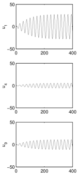
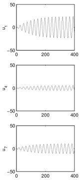
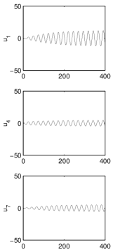
	B	C

Figure 3: Pattern selectivity:  A: Response evoked on 3 of the 10 neurons of the network by input patterns a, b, and c matching the imprinted pattern a in frequency. The class I activation functions shown in Fig.1BD have been used.  B: Response amplitude $|\langle{\bf u}^{+}|\boldsymbol{\xi}^{\mu}{\rm e}^{-{\rm i}\omega_{\mu}t}\rangle|$ vs. input overlap $|\langle\boldsymbol{\xi}{{}^{{\mu}}}|\boldsymbol{\xi}\rangle|$, under input $\delta{\bf I}^{+}=\boldsymbol{\xi}{\rm e}^{-{\rm i}\omega_{{\mu}}t}$. Results from linearized theory (solid line) and from models with class I (stars) and II (circles) nonlinearities.  C: Hysteresis effects in class II simulations. The response amplitude depends on the history of the system: the output remains at the resonance level after input withdrawl (circles connected by dotted line). Circles connected by solid line correspond to the case of random or zero-overlap initial conditions. The connecting lines are drawn for clarity only.

3.2.3 Interpolation and categorization.

With multiple imprinted patterns, an input $\delta{\bf I}^{+}=\xi{\rm e}^{-{\rm i}\omega t}$ which overlaps with several of them will evoke a correspondingly mixed resonant linear response ${\bf u}^{+}=\chi(\omega;\omega_{\mu})\delta{\bf I}^{+}_{{\|}}+\chi_{0}(\omega)\delta{\bf I}^{+}_{\perp}$, where $\delta{\bf I}^{+}_{\|}=\sum_{\mu}\langle\boldsymbol{\xi}^{\mu}|\boldsymbol{\xi}\rangle\boldsymbol{\xi}^{\mu}{\rm e}^{-{\rm i}\omega t}$. That is, any input in the pattern subspace produces a resonant linear response just like that to an input proportional to a single pattern. This is a standard property of linear associative memories for orthogonal patterns. (We remind the reader that when the number of patterns is much smaller than the number of units in the network, independent random patterns may be taken as effectively orthogonal.) This feature enables the system to interpolate between imprinted patterns, i.e., to perform an elementary form of generalization from the learned set of patterns. This property can be useful for input representation.

A similar property also holds in the class I nonlinear model, but not in the class II model. To see this, suppose the drive ${\bf I}=\boldsymbol{\xi}e^{-{\rm i}\omega_{\mu}t}+{\rm c.c.}$ overlaps two imprinted patterns, with $\boldsymbol{\xi}\propto\boldsymbol{\xi}^{1}\cos\psi+\boldsymbol{\xi}^{2}\sin\psi$, and write the response ${\bf u}^{+}$ as ${\bf u}^{+}\propto\boldsymbol{\xi}^{1}\cos\phi+\boldsymbol{\xi}^{2}\sin\phi$. For a linear model, $\phi=\psi$. The class I nonlinear model gives $45^{o}\geq\phi>\psi$ when $\psi<45^{o}$ and $45^{o}<\phi<\psi$ when $\psi>45^{o}$ (see Fig. 4). Thus, it tends to equalize the response amplitudes to $\boldsymbol{\xi}^{1}$ and $\boldsymbol{\xi}^{2}$ even when they contribute unequally to the input. In contrast, the class II nonlinear model amplifies the difference in input strengths to give higher gain to the stronger input component, $\boldsymbol{\xi}^{1}$ or $\boldsymbol{\xi}^{2}$, thus performing a kind of categorization of the input. Thus, the two nonlinearity classes leads to different computational properties. For the case shown in Fig. 4B the parameters are such that the categorization is into three categories, corresponding to outputs near $\xi^{1}$, $\xi^{2}$, and their symmetric combination. For stronger nonlinearity, bipartite classification is possible.

Figure 4: A, B: Input-output relationship when two orthogonal patterns, $\boldsymbol{\xi}^{1}$ and $\boldsymbol{\xi}^{2}$, have been imprinted at the same frequency $\omega_{\mu}=41Hz$. Input $\boldsymbol{\xi}\propto\boldsymbol{\xi}^{1}\cos\psi+\boldsymbol{\xi}^{2}\sin\psi$ and response ${\bf u}\propto\boldsymbol{\xi}^{1}\cos\phi+\boldsymbol{\xi}^{2}\sin\phi$. Circles show the simulation results, dotted lines show the analytical prediction for the linearized model. A: Class I. B: Class II. C: Categorization using different imprinting frequencies. Plotted are responses of 3 of the 10 excitatory units to various input patterns and frequencies. Patterns $\boldsymbol{\xi}^{1}{\rm e}^{-{\rm i}\omega_{1}t}$ and $\boldsymbol{\xi}^{2}{\rm e}^{-{\rm i}\omega_{2}t}$, where $\boldsymbol{\xi}^{1}\perp\boldsymbol{\xi}^{2}$, $\omega_{1}=41$ Hz and $\omega_{2}=63$ Hz, have been imprinted. Matched kernels are used with $\tilde{A}_{J}(\omega_{1})=0.5-0.025{\rm i}$ and $\tilde{A}_{J}(\omega_{2})=0.5-0.43{\rm i}$ satisfying resonance conditions. For the mixed input (fourth column), $a=1/\sqrt{17}$ and $b=4/\sqrt{17}$.

Another way to prevent undesirable interpolation between imprinted patterns (or classes of them) is to store different patterns or classes at frequencies that differ by more than the frequency tuning width. Suppose $\boldsymbol{\xi}^{1}{\rm e}^{-{\rm i}\omega_{1}t}$ and $\boldsymbol{\xi}^{2}{\rm e}^{-{\rm i}\omega_{2}t}$ are imprinted, with $\omega_{1}\neq\omega_{2}$ and $\boldsymbol{\xi}^{1}\cdot\boldsymbol{\xi}^{2}\approx 0$. Then we have $J_{ij}=J_{ij}^{1}+J_{ij}^{2}$ and $W_{ij}=W_{ij}^{1}+W_{ij}^{2}$, where $J_{ij}^{\mu}$ and $W_{ij}^{\mu}$ are given by equations (14) with corresponding frequencies for $\mu=1,2$. The resonance and stability conditions should be enforced separately for each pattern.

After learning, an input ${\bf I}^{+}=(\boldsymbol{\xi}^{1}+\boldsymbol{\xi}^{2}){\rm e}^{-{\rm i}\omega_{1}t}$ at frequency $\omega_{1}$ will evoke a response

$${\bf u}^{+}\approx\chi(\omega_{1},\omega_{1})\boldsymbol{\xi}^{1}+\chi(\omega_{1},\omega_{2})\boldsymbol{\xi}^{2}\approx\chi(\omega_{1},\omega_{1})\boldsymbol{\xi}^{1}$$ (43)

since $\chi(\omega_{1},\omega_{2})\ll\chi(\omega_{1},\omega_{1})$ by design when $|\omega_{1}-\omega_{2}|\ll\Delta$. Hence, as illustrated in Fig. 4C, the system filters out the oscillation patterns learned at a different oscillation frequency from the input frequency.

4 Nonlinear analysis

Nonlinearity affects the response mainly at large amplitudes, which occur during resonant recall but not (we assume) in learning mode. Hence, in the following analysis, we leave the formulae for ${\sf J}$, ${\sf W}$, and ${\sf M}$ unchanged, ignore nonlinearity in response components orthogonal to the pattern subspace, and examine the corrections to the linear response ${\bf u}=\chi(\omega;\omega_{\mu})\delta{\bf I}_{\|}$. We take the input to be along the imprinted pattern $\boldsymbol{\xi}^{\mu}$: $\delta{\bf I}^{+}_{\|}=I\boldsymbol{\xi}^{\mu}{\rm e}^{-{\rm i}\omega t}$. We focus on the nonlinearity in $g_{u}$, since $g^{\prime}_{v}$ only affects the local synaptic input, while $g^{\prime}_{u}$ also affects the long-range input. Equation (7) then becomes

$$[(\alpha-{\rm i}\omega)^{2}]{{\bf u}}={{\sf M}}g_{u}({\bf u})+(\alpha-{\rm i}\omega)\delta{\bf I}.$$ (44)

where for simplicity, we include $\gamma$ as a diagonal element of $\sf W$, and by $g_{u}({\bf u})$ we mean a vector with components $[g_{u}({\bf u})]_{i}=g_{u}(u_{i})$. Making the ansatz ${\bf u}={q}\boldsymbol{\xi}^{\mu}{\rm e}^{-{\rm i}\omega t}+{\rm c.c.}+$ higher order harmonics, we have,

$$u_{j}^{3} \approx 3{q^{2}q^{*}}{\xi^{\mu}_{j}}^{2}\xi^{\mu*}_{j}{\rm e}^{-{\rm i}\omega t}+{\rm c.c.}+\;\;\mbox{higher order harmonics},$$ (45)

and analogously for $u_{j}^{5}$. The quantity $q$ is the response amplitude of interest; in the linearized theory $q\rightarrow\chi(\omega;\omega_{\mu})I$.

For the two nonlinearity classes (9) we have, respectively,

$${\sf M}\,g({\bf u}) {\approx} \left(1-{3a|{q}|^{2}}\sum_{j}{|\xi^{\mu}_{j}|}^{4}\right){\sf M}{\bf u},$$ (46)

$${\sf M}\,g({\bf u}) {\approx} \left(1+{3a|{q}|^{2}}\sum_{j}{|\xi^{\mu}_{j}|}^{4}-{5b|{q}|^{4}}\sum_{j}{|\xi^{\mu}_{j}|}^{6}\right){\sf M}{\bf u}.$$ (47)

Thus, at a given response strength $|q|$, the imprinting strengths are effectively multiplied by the factors in parentheses. Consequently, class I nonlinearity reduces the response at large amplitude, whereas class II nonlinearity enhances it as long as the quadratic term in $|q|$ is larger than the quartic one.

A consequence for class II is the fact that a system which is very close to resonance ($\epsilon,\Delta\rightarrow 0$) in the linear regime can become unstable at higher response levels. The system will then jump to a new state in which the (negative) quartic term in (47) is large enough that stability is restored, as seen in Figs. 2 and 3

Substituting (46) and (47) into (44) and matching the coefficients of $\boldsymbol{\xi}^{\mu}{\rm e}^{-{\rm i}\omega t}$ on left and right sides, we obtain, for the two nonlinearity classes, respectively,

$$\chi^{-1}(\omega;\omega_{\mu})q+{3aB}\sum_{j}|\xi^{\mu}_{j}|^{4}|{q}|^{2}{q}=I,$$ (48)

$$\chi^{-1}(\omega;\omega_{\mu})q-{3aB}\sum_{j}|\xi^{\mu}_{j}|^{4}|{q}|^{2}{q}+{5bB}\sum_{j}|\xi^{\mu}_{j}|^{6}|{q}|^{4}{q}=I.$$ (49)

where $B\equiv\Pi(\omega;\omega_{\mu})/(\alpha-{\rm i}\omega)$. These equations can be solved for $q$. It is apparent that in general, both the phase and the amplitude of $q$ are modified by the nonlinearity.

5 Effects of synaptic weight constraints

Because of the excitatory character of the pre-synaptic unit, $J_{ij}$ and $W_{ij}$ connections have to be non-negative, a condition not respected by our learning formula (14) so far. As a remedy, one may (1) add an initial background weight, $\bar{J}/N$ or $\bar{W}/N$, independent of $i$ and $j$, to each connection to make it positive, i.e.,

$$\left\{\begin{array}[]{l}J_{ij}=\bar{J}/N+\sum_{\mu}2{\rm Re}\,[\tilde{A}_{\rm J}\xi_{i}^{\mu}\xi_{j}^{\mu*}]/N\geq 0\\ W_{ij}=\bar{W}/N+\sum_{\mu}2\gamma{\rm Re}\,\left[\frac{\tilde{A}_{\rm W}\xi_{i}^{\mu}\xi_{j}^{\mu*}}{\alpha-{\rm i}\omega_{\mu}}\right]/N\geq 0.\\ \end{array}\right.$$ (50)

and/or (2) delete all net negative weights.

It is clear from equations (50) that adding a background weight is like learning an extra pattern $\boldsymbol{\xi}^{0}$ that is uniform and synchronous, with $\xi^{0}_{i}=1$ for all $i$, with learning kernels $\tilde{A}^{(0)}_{J}(\omega_{0})$ and $\tilde{A}^{(0)}_{W}(\omega_{0})$ which satisfy $2{\rm Re}\,\tilde{A}^{(0)}_{J}(\omega_{0})$ = 1 and $2\gamma{\rm Re}\,[A^{(0)}_{W}(\omega_{0})/\alpha-{\rm i}\omega_{0}]=1$. We assume that these kernels are the same as those with which the patterns $\xi_{i}^{\mu}$ are imprinted, up to an overall learning strength factor: $\tilde{A}^{(0)}_{J,W}(\omega)=\eta\tilde{A}_{J,W}(\omega)$, and that the imprinting frequencies are the same: $\omega_{\mu}=\omega_{0}$. Thus if the $\xi_{i}$ are of unit magnitude, in order to guarantee that no $J_{ij}$ or $W_{ij}$ are to be negative we need $\eta\geq 1$.

This strategy can be effective provided that the imprinting of the uniform extra pattern does not lead to violation of any stability condition. Since we have assumed the imprinted patterns $\boldsymbol{\xi}^{\mu}$ ($\mu>0$) are (roughly) orthogonal to $\boldsymbol{\xi}^{0}$, we can treat the extra pattern independently of the others, and we just have to satisfy the same stability conditions for it that we previously found for the imprinted patterns. That is, the singularities of $\chi(\omega;\omega_{\mu})$ have to lie in the lower half of the $\omega$ plane, where now $\chi(\omega;\omega_{\mu})$ (Eqn. 22) has to be computed from a $\Pi(\omega;\omega_{\mu})$ which is a factor $\eta$ larger than before. For $\eta\rightarrow 1$, we get no change in the stability conditions.

Nonnegativity can be more practically achieved by simply deleting the net negative weights. For random patterns, and without background weights $\bar{J}$ and $\bar{W}$, this leads to deleting half of the weights $J_{ij}$ and $W_{ij}$ obtained from the learning rule, which weakens their effect, quantified by the function $\Pi(\omega;\omega_{\mu})$, by a factor of 2. In simulations we have found that increasing the learning strength by this factor leads to results like those found earlier when negative $J_{ij}$ and $W_{ij}$ were permitted.

Finally, we remark that negative weights can also be simply implemented via inhibitory interneurons with very short membrane time constants.

6 Summary and Discussion

6.1 Summary

We have presented a model of learning and retrieval for associative memory or input representation in recurrent neural networks that exhibit input-driven oscillatory activities. The model structure is an abstraction of the hippocampus or the olfactory cortex. The learning rule is based on the synaptic plasticity observed experimentally, in particular, long-term potentiation and long-term depression of the synaptic efficacies depending on the relative timing of the pre- and postsynaptic spikes during learning. After learning, the model’s retrieval is characterized by its selective strong responses to inputs that resemble the learned patterns or their generalizations. Our work generalizes the outer-product Hebbian learning rule in the Hopfield model to network states characterized by complex state variables, representing both amplitudes and phases. Our work differs from previous modeling in the following respects: (1) We allow that stored patterns vary in both amplitudes and phases, as well oscillation frequency. (2) We imprint input patterns into the synapses using a generalized Hebbian rule that gives LTP or LTD according to the relative timing of pre- and postsynaptic activity. (3) We explore two qualitatively different functions of the network: one (associative memory) is to classify inputs into distinct categories corresponding to the individual learned examples, and the other is to represent inputs as interpolations between or generalizations of learned examples.

The same model structure was used previously, with a conventional Hebbian rule with $A_{J,W}(\tau)\propto\delta(\tau)$, by two of the authors in a model for odor recognition/classification and segmentation in the olfactory cortex[10]. The principal new contributions in the current work are (1) linking the model with the recent experimental data on neural plasticity and LTP/LTD and dissecting the role of the functional form of the learning kernel $A_{J,W}(\tau)$ in determining the selectivity to input patterns and frequencies, (2) an extended analysis of input selectivity and tuning, (3) exploration of the two different computational functions (associative memory and input representation) of the model, and (4) a detailed analysis of nonlinearity in the model.

6.2 Discussion

By using both amplitude and phase to code information, it is possible either to encode additional information or to increase robustness by redundantly coding the same information coded by the amplitudes. Indeed, hippocampal place cells, which code the spatial location of the animal, fire at different phases of the theta wave depending on the location of the animal in the place fields[14]. In this case, the information encoding is redundant since the location is in principle already encoded by the firing rates (i.e., oscillation amplitudes) in the neural population. In our model, combined phase and amplitude coding requires matching both the amplitude and phase patterns of the inputs with the learned inputs under recall, making matching more specific. This scheme necessitates learning both excitatory-to-excitatory connections and excitatory-to-inhibitory ones. Thus, in a system of $N$ coupled oscillators, the stored items are coded by $2N$ variables — $N$ amplitudes and $N$ phases, requiring the specification of $2N^{2}$ synaptic strengths — $N^{2}$ excitatory-to-excitatory synapses and another $N^{2}$ excitatory-to-inhibitory ones. Omitting phase coding would require learning of only $N^{2}$ synapses, e.g., of the excitatory-to-excitatory connections, as in previous models[15, 16].

Our model’s frequency selectivity adds additional matching specificity during recall. Furthermore, frequency matching can modulate the spiking timing reliability, since higher or lower oscillation amplitudes, caused by better or worse frequency matching, should make the firing probabilities of the cells more or less modulated or locked by oscillation phases. Frequency dependence of spike timing reliability has been observed in cortical pyramidal cells and interneurons [17]. In our model, the frequency tuning is a network property imprinted in long-range connections, although frequency tuning as a resonance phenomenon could in principle exist in a single neural oscillator or a local circuit.

In our model, both excitatory-to-excitatory and excitatory-to-inhibitory synapses are modifiable. Experimentally, there is as yet little evidence concerning plasticity in pyramidal-to-interneuron synapses. More experimental investigations are needed. In experiments by Bell [5], plasticity of the excitatory-to-inhibitory synapses between parallel fibers and medium ganglion cells in the cerebellum-like structure of the electric fish has been observed. although these synapses are not part of a recurrent oscillatory circuit.

We explored the constraints on the learning kernel functions $A_{J,W}(\tau)$ imposed by the requirement of a resonant response. A condition that came up in almost all the variants of the model that we explored was that $\tilde{A}_{J}^{\prime}(\omega_{\mu})$ should be positive in order to achieve a strong, narrow resonance. This means, roughly, that for excitatory-excitatory synapses LTP should dominate LTD in overall strength, for spike time differences smaller than $1/\omega_{\mu}$.

Another condition we considered was that the resonant frequency should be the same as the driving frequency $\omega_{\mu}$ during learning. We saw that for real patterns and learning only of the excitatory-excitatory connections, this could not be satisfied for general $\omega_{\mu}$. However, with learning of the excitatory-to-inhibitory connections it could, for a suitable (negative) value of $\tilde{B}^{\prime\prime}_{W}(\omega_{\mu})$. For complex patterns (see Eqn. 29), the imaginary parts of both $\tilde{B}_{J}$ and $\tilde{B}_{W}$ contribute to the shift, so if they have opposite signs (of the correct relative magnitude) the condition can be satisfied, independent of $\omega_{\mu}$. These features should be looked for in investigations of plasticity of excitatory-to-inhibitory synapses.

An interesting property we have identified in the model is its ability to subserve two different computational functions: to classify inputs into distinct learned categories, and to represent input patterns as interpolation and generalizations of the prototype examples learned.

Categorization is appropriate for associative memories and has been applied in our previous model of olfactory cortex[10]. In this context, interpolation between different learned patterns is not desired; individually learned odors should have specific roles. It is more desirable to perceive individual odors within an odor mixture than to perceive an unspecific blend.

On the other hand, interpolation is advantageous in some circumstances. Consider an animal learning an internal representation of a region of space. If particular spatial locations are represented as particular imprinted patterns, then locations in between them will be represented as linear combinations of these patterns. Thus, the network is able to represent a continuum of positions in a natural way. Hippocampal place cells seem to employ such a representation. A network that interpolates can generalize from the learned place fields to represent spatial locations between the learned place fields by superposition of the neural activities of the place cells. Because the place fields are localized, the generalization is conservative (and thus robust): It does not extend beyond the spatial range of the learned locations or to regions between distant, disjoint place fields.

We showed that our network can serve one or the other of these two computational functions, depending on the nonlinearity in the neuronal activation functions. Class I leads to the interpolation or input representation operation mode, while class II leads to categorization. The form of $g(u)$ could be subject to modulatory control, permitting the network to switch function when appropriate. The switch could even be accomplished, for a suitable form of $g(u)$, simply by a change in the DC input level, since it is possible to change the effective nature of the nonlinearity near the operating point by shifting the resting point. It seems likely to us that the brain may employ different kinds and degrees of nonlinearity in different areas or at different times to enhance the versatility of its computations.

We have seen that it is possible to store different classes of patterns at different oscillation frequencies, and that the network does not interpolate between patterns stored at different frequencies. This feature gives the system the possibility of performing several different forms of input representation or categorization without interference between them. For instance, all place fields could be stored at one frequency, while odor memories could be stored at another, and there would be no crosstalk between the two modalities if the frequencies differed by much more than the resonance linewidth.

In conclusion, we have seen that this rather simple network is endowed with interesting computational properties which are consequences of the combination of its oscillatory dynamics and the spike-timing-dependent synaptic modification rule. Although experiments to date have not clearly uncovered examples of networks in the brain that function in just this fashion, we hope that our findings here will stimulate further investigations, both theoretical and experimental.

References

- [1] Magee J.C., and Johnston D. Science 275 p.209, 1997.
- [2] Debanne D., Gahwiler B.H. and Thompson S.M. J. Physiol. 507, p.237, 1998.
- [3] Bi G.Q., and Poo M.M. J. Neurosci. 18 p.10464, 1998.
- [4] Markram H., Lubke J., Frotscher M., Sakmann B. Science 275 p.213, 1997.
-
[5]
Bell CC, Han VZ, Sugawara Y, Grant K
Nature 387 (6630), p.278-81, 1997
Bell C.C., Han V.Z., Sugawara Y., Grant K. Jour. of Exper. Biology 202 , p. 1339-1347, 1999. - [6] Feldman D.E. Neuron 27, p.45-56, 2000.
- [7] Debanne D., Gahwiler B.H., Thompson S.M. Proc. Nat. Acad. Sci. USA 91, 1148-1152, 1994.
- [8] Li Z., Dayan P. Network: Computation in Neural Systems 10, p.59, 1999.
- [9] Hertz, J. A., Krogh, A., and Palmer, R. G., Introduction to the Theory of Neural Computation Addison-Wesley, 1991.
- [10] Li Z. and Hertz J., Network: Computation in Neural Systems 11, p.83-102, 2000.
- [11] Kempter R., Gerstner W. and van Hemmen L. Physical Review E vol. 59, num. 5, p.4498, 1999.
-
[12]
Hasselmo M. E.,
Neural Computation 5, p.32-44 (1993).
Hasselmo M.E. Trend in Cognitive Sciences, Vol.3, No.9, p.351 (1999). - [13] Amit, D. J., Gutfreund, H., and Sompolinsky, H., Phys. Rev. Lett., 55, p. 1530, 1985.
- [14] J. O. Keefe and M. L. Recce, Hippocampus, vol 3, n.3, p. 317-330, 1993
- [15] Hendin O., Horn D., Tsodyks MV. J Comput Neurosci. 5(2): p.157-69, 1998.
- [16] Wang D.L., Buhmann J., and von der Malsburg C. Neural Comput. 2. 94-106, 1990
- [17] J. M. Fellous, A. R. Houweling, R. H. Modi, R. P. N. Rao, P. H. E. Tiesinga, and T. J. Sejnowski. Journal of Neurophysiology, p. 1782-1787, 2001.