Mode-Coupling Theory of Colloids with Short-range Attractions

Abstract

Within the framework of the mode-coupling theory of super-cooled liquids, we investigate new phenomena in colloidal systems on approach to their glass transitions. When the inter-particle potential contains an attractive part, besides the usual repulsive hard core, two intersecting liquid-glass transition lines appear, one of which extends to low densities, while the other one, at high densities, shows a re-entrant behaviour. In the glassy region a new type of transition appears between two different types of glasses. The complex phenomenology can be described in terms of higher order glass transition singularities. The various glass phases are characterised by means of their viscoelastic properties. The glass driven by attractions has been associated to particle gels, and the other glass is the well known repulsive colloidal glass. These correspondences, in associations with the new predictions of glassy behaviour mean that such phenomena may be expected in colloidal systems with, for example, strong depletion or other short-ranged attractive potentials.

1 Introduction

The experimental study of the glass transition in colloidal systems [1] has been a very important test case to assess the validity of theories concerning the formation of an amorphous solid from super-cooled liquids. In particular the mode-coupling theory (MCT) has been useful when applied to colloids, modeled as spherical particles interacting through a hard sphere purely repulsive potential [2]. In this case the MCT predicts the existence of a critical volume fraction $\phi$ where the system undergoes an ergodic-nonergodic transition, which was observed experimentally using quasi-elastic dynamic light scattering [3]. From the physical point of view the MCT describes in a fairly accurate way the so-called cage effect, i.e. the fact that at high densities molecular motions of particles are constrained by the presence of the surrounding ones which form a cage around each particle. Prior to reaching the MCT transition, we may think of the particle vibrating within their cages at short time-scales, and escaping from their cages at somewhat longer time-scales. The two time scales show up in a well-defined way, when the liquid system gets closer to the critical threshold, as distinct relaxation regimes separated by a plateau region which becomes more and more extended as criticality is approached. Close and above the plateau, there is a power law and the plateau ends with another power law prior to enter into the so-called full $\alpha$ regime. The power-law region is called $\beta$ correlator in the framework of $MCT$. The $\alpha$ decay is quite well phenomenologically described by a stretched exponential.

We have briefly sketched the main features of the MCT for colloids considered as hard spheres and proceed to consider the novel consequences of adding an attractive contribution to the inter-particle potential. In this paper we mainly consider the effects of using a hard core followed by a square well potential in order to mimic the interactions between colloidal particles. In real systems this can be obtained, for example, by covering the surface of the particles with a polymer coating or with depletion interaction [4]. A description of such systems using the MCT approach has revealed the existence of a set of new and interesting phenomena, that we briefly summarise in what follows [5, 6]. In the temperature $T$ and volume fraction $\phi$ plane MCT predicts two lines of transition from liquid to glass.One of the lines extends to high temperatures, it can be traced essentially to the repulsive part of the potential and tends asymptotically for high temperatures to the value $\phi$ corresponding to the critical value for hard spheres. We will call it the repulsive glass transition line (RGL). On lowering the temperature the transition line moves toward higher values of $\phi$ and gives rise to a re-entrant behaviour, i.e. one can pass from a liquid to a glassy state either by lowering or by raising $T$. In other words the liquid phase tends to exist in a region which extends more deeply into the glassy phase compared to the hard spheres case. The origin of this unusual effect is that if the interaction is short ranged enough, there can, in this temperature and density regime, be partial cancellation of the repulsive and attractive interactions leading to a phenomenon for glasses, not unlike that of a theta point for polymers.

The other glass transition line, originating in a relatively well-defined energy scale of the well-depth, is almost parallel to the $\phi$ axis and extends on one side of the binodal to the other, until it eventually crosses the repulsive transition line. We call it the attractive glass transition line (AGL). For sufficiently narrow well-widths and on the high $\phi$ end the AGL enters the glass region and terminates in an endpoint. Thus the two sides of the line separate two different types of glassy system that we will characterise through their mechanical properties. The endpoint of the AGL is a higher order glass transition point (called $A_{3}$), which will be shown to have special dynamical properties, namely the relaxation slows down dramatically on approaching it. Upon increasing the width of the potential well, the length of the AGL shrinks and its extension into the glass region reduces to zero, and as a consequence the endpoint turns into a higher transition point (called $A_{4}$). We will characterise this rather complex behaviour of the system, where repulsion and attraction compete, using two typical dynamical quantities, the shear viscosity, which characterises the liquid phase, and the elastic shear modulus for the amorphous glass.

Aspects of the MCT have been tested in many different cases, both experimentally and with computer molecular dynamics [7]. The most extensive and accurate experimental check has been performed in the liquid-glass transition of colloidal systems, treated as hard sphere systems, and studied with dynamic light scattering [3]. The agreement with MCT is quantitatively satisfactory [8]. In a similar fashion computer simulations have been used to study the glass transition in simple model systems, as diverse as Lennard-Jones binary systems [9], the SPC/E model for water [10], orthoterphenil [11] and silica [12]. In all these cases evidence shows that these systems undergo a kinetic glass transition, and the molecular dynamics is well accounted for by the idealised MCT of super-cooled liquids. On the other hand there is extensive evidence, mainly due to experimental results in colloidal systems, that cannot be interpreted in terms only of hard-core potentials.

Dense systems of colloidal particles characterised by a hard core and strong short-ranged attractions have been realized experimentally by adding polymers to either a suspension of colloidal hard spheres [4], in solutions of sterically stabilised particles when decreasing the solvent quality [13], and in copolymer micellar systems when changing the temperature [14]. Such systems were also studied by Monte Carlo simulations [15]. The facts that cannot be simply explained using hard-core potentials are the following.

(i) An amorphous material can be formed by increasing the attraction strength even though the volume fraction is kept well below the value of the hard sphere glass transition [13, 16, 17, 18, 19].

(ii) In mixtures of colloids and polymers, melting of the glass states is obtained by increasing the strength of a short range attraction by the addition of small polymers [4].

(iii) Using solvents of decreasing quality [13] in polymer coated colloidal particles the long time limit of the density time correlation function at small wave vectors are much larger than in hard-sphere systems.

(iv) Viscoelastic measurements for intermediate frequencies found strongly concentration dependent elastic moduli [16, 17, 18, 19].

(v) A system in which an anomalous dynamical behaviour has been reported is a polymer solution (called L64) where structural arrest accompanied by a logarithmic-like decay of the density correlator is observed [20].

The paper is organised as follows. In Section 2 we report the details of the calculation of the structure factor for a square-well system (SWS), the only input needed for the mode-coupling dynamics, which is described in Section 3. The resulting phase diagram is described in Section 4, the time dependent density correlation functions in Section 5 and finally the various phases are characterised by their mechanical properties in Section 6. In Section 7 we report our conclusions.

2 Calculation of the structure factor

In the framework of the MCT the only quantity that is needed in order to calculate the dynamical properties of a super-cooled liquid approaching the glass transition is the structure factor. It is well known that, given an inter-particle potential satisfying the Ornstein-Zernike equation for the space-dependent pair correlation function $g(r)$, one needs a closure approximation in order to solve the equation. Many approximations of this type have been proposed and solved in the case of simple model potential [21]. In the case of the square-well potential the Wiener-Hopf method as formulated by Baxter [22] can be used. The interaction potential $V(r)$ for particles a distance $r$ apart, is obtained with a hard-core repulsion for $r<d$, and the negative attractive value $-u_{0}$ within the range $d<r<sD$.

The structure factor is specified by three control parameters, i.e. the packing fraction $\phi$ related to the hard cores, the temperature $T$, and the relative width $\epsilon=1-d/D$ of the attraction shell. In the Baxter approach the structure factor $S_{q}$ is expressed in terms of the Fourier transform $\widetilde{Q}(q)$ of the factor function $Q(r)$, a continuous real function defined for $r\geq 0$,

$$S_{q}^{-1} = \widetilde{Q}(q)\widetilde{Q}^{*}(q)\,,$$ (1)

$$\widetilde{Q}(q) = 1-2\pi\rho\int_{0}^{\infty}{d}r\exp(iqr)Q(r)\,.$$ (2)

The funcion $Q(r)$ is related to the direct correlation function $c(r)$ [21] and both functionss vainsh beyond the distance $D$. For $0\leq r\leq D$, the following equation for $Q(r)$ holds

$$rc(r)=-Q^{\prime}(r)+2\pi\rho\int_{r}^{R}{d}s\,Q^{\prime}(s)Q(s-r)\,.$$ (3)

In addition for $r>0$

$$rh(r)=-Q^{\prime}(r)+2\pi\rho\int_{0}^{R}{d}s(r-s)h(|r-s|)Q(s)\,.$$ (4)

For the SWS, $g(r)=0$ is fulfilled for $0<r<d$, and therefore, using $h(r)=g(r)-1$, equation (4) splits into three sub-equations. The result for the middle part, $\Delta\leq r\leq d$, where $\Delta=D-d$, is very simple since the formula known from the theory for the hard-sphere system is reproduced

$$Q^{\prime}(r)=ar+b\,,$$ (5)

where the coefficients $a$ and $b$ are introduced by

$$a=1-2\pi\rho\int_{0}^{d+\Delta}{d}s\,Q(s)\,,\quad b=2\pi\rho\int_{0}^{d+\Delta}{d}s\,s\,Q(s)\,.$$ (6)

Defining $G(r)=rg(r)$ one finds, for small distances, $0\leq r\leq\Delta$, where $\Delta=D-d$,

$$Q^{\prime}(r)=ar+b-2\pi\rho\int_{r+d}^{d+\Delta}{d}s\,G(s-r)Q(s)\,,$$ (7)

and for the attraction shell, $d\leq r\leq D$, one obtains

$$Q^{\prime}(r)=ar+b-G(r)+2\pi\rho\int_{0}^{r-d}{d}s\,G(r-s)Q(s)\,.$$ (8)

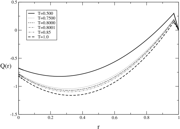
Figure 1: The Baxter factor function $Q(r)$ at $\epsilon=0.03$, $\phi=0.504449$ and different temperatures. The hard-core diameter is chosen as the unit of length.

A closure approximation for $c(r)$ must be introduced into equation (3) in order to complete the system of equations (3) and (8). Using the Percus-Yevick (PY) approximation [21], according to which

$$c(r)=g(r)\left[1-exp\left({{V(r)}\over{k_{B}T}}\right)\right]$$ (9)

inside the hard core in equation (3) and equation (8) leads to the approximation valid for $d\leq r\leq d+\Delta$

$$e^{-u_{0}/k_{B}T}G(r)= ar+b-2\pi\rho\int_{r}^{d+\Delta}{d}s\,Q^{\prime}(s)Q(s-r)$$ (10)

$$+2\pi\rho\int_{0}^{r-d}{d}s\,G(r-s)Q(s)\,.$$

Equations (8) and (10) for $Q(r)$ and $G(r)$ are solved numerically choosing on each of the three intervals of the variable a grid of equally spaced points $r_{n}$, where $n=1,2,\dots,1000$. The integral in equation (2) is then performed to obtain $\widetilde{Q}(q)$ and hence $S_{q}$. The typical values for the factor function $Q(r)$ are shown in figure 1, while figure 2 shows the corresponding structure factors $S_{q}$ for various temperatures, given in term of the well depth $u_{0}$ as $k_{b}T/u_{0}$.

In a first attempt to solve the problem associated with the attractive part of the inter-particle potential the Baxter potential has been used [22], i.e. the limit of a square-well in which the range of the potential vanishes while its depth increases in such a way that their product remains constant [5]. The mean spherical approximation has also been used in conjunction with an attractive Yukawa potential in an attempt to explain colloidal gelation [23]. We may note that more recently other methods of generating the structure factors have been explored [6, 24]. The main results reported here are found not to depend on these details, and we therefore here only comment on the square well potential.

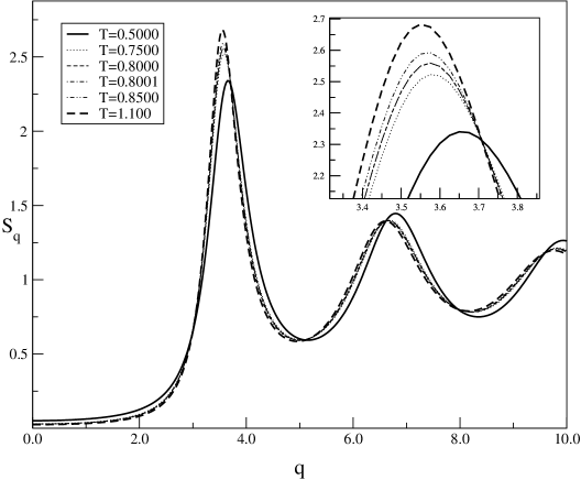
Figure 2: The structure factors function in the PY approximation at various temperatures, $\epsilon=0.03$ and $\phi=0.504449$. The inset shows the maxima of the structure factors.

3 The mode-coupling equations

The MCT of the ideal liquid-glass transition is capable of describing the ergodic to non-ergodic transition in the normalised density correlation function

$$\phi_{q}(t)={{\langle\rho_{{\vec{q}}}^{*}(t)\rho_{\vec{q}}\rangle}\over{\langle|\rho_{\vec{q}}|^{2}\rangle}}.$$ (11)

In the long time limit $\phi_{q}(t)$ shows a discontinuous variation from a vanishing value in a super-cooled liquid to a finite value different from zero $f_{q}$ in a glassy state, on varying the external control parameters. In the latter state the system experiences a structural arrest. In real systems the transition point is never reached since new dynamical mechanisms set in which bypass the ergodicity breakdown. The MCT equations are

$$\ddot{\phi_{q}}(t)+\Omega_{q}^{2}\phi_{q}(t)+\nu_{q}\dot{\phi_{q}}(t)+\Omega_{q}^{2}\int_{0}^{t}m_{q}(t-t^{\prime})\dot{\phi_{q}}(t^{\prime})dt^{\prime}=0$$ (12)

where the mode-coupling memory functional $m_{q}$ is given by

$$m_{q}(f)=\frac{1}{2}\int{{{{d}^{3}k}\over(2\pi)^{3}}V_{\vec{q},\vec{k}}f_{k}f_{|\vec{q}-\vec{k}|}}\,.$$ (13)

The mode-coupling vertices are determined by the density $\rho$, the structure factor $S_{q}$ and the direct correlation function $c_{q}=(1-1/S_{q})/\rho$

$$V_{\vec{q},\vec{k}}\equiv S_{q}S_{k}S_{|\vec{q}-\vec{k}|}{\rho\over{q^{4}}}\left[{\vec{q}}\cdot\vec{k}\,{c_{k}}+\vec{q}\cdot(\vec{q}-\vec{k})\,{{c_{|\vec{q}-\vec{k}|}}}\right]^{2}\,.$$ (14)

The two quantities $\Omega_{q}$ and $\nu_{q}$ are respectively the characteristic frequency of the phonon-type motions of the fluid, and a term that describes instantaneous damping arising from the fast contribute to the memory function. They are defined as

$$\Omega_{q} = \frac{q^{2}k_{B}T}{mS(q)}$$

$$\nu_{q} = \nu_{1}q^{2}$$

and $\nu_{q}=1$ in our calculations. In the long time limit $t\rightarrow\infty$, the density correlators $\phi_{q}(t)$ tend to a value

$$f_{q}={{\langle\rho^{*}_{q}(0)\rho_{q}(\infty)\rangle}\over{\langle|\rho_{q}(0)|^{2}\rangle}}$$ (15)

the non-ergodicity factor, or Debye-Waller factor. The MCT equations (12) in the static limit give rise to the bifurcation relation

$$\frac{f_{q}}{1-f_{q}}=\frac{1}{2}\int\!\!\frac{d^{3}k}{(2\pi)^{3}}\,\,V({\bf q},{\bf k})f_{k}f_{|{\bf q}-{\bf k}|}$$ (16)

It is clear that $f_{q}=0$ is a solution of equations (16) and it corresponds to an ergodic state of the system in which the correlations decay for long time. The correlators tend instead to a finite value different from zero if the system is kinetically arrested. This loss of ergodicity for $\phi$ is interpreted as the transition to a kinetic glassy state. Therefore for some critical values of the thermodynamic parameters, density and temperature in our case, bifurcations of the solutions of the asymptotic equations appear that produce non-zero solutions. The bifurcations can be multiple, up to the number of control parameters of the system. Thus, when a bifurcation gives rise to more than two solutions of equations (16), there will exist multiple solutions with finite non-ergodicity factors. In these cases one speaks of $A_{k}$-type bifurcations, with $k=2,3,4,\dots$ In this case, MCT predicts that only the state corresponding to the largest value of $f_{q}$ is a stable solution of the equations [2].

4 Phase diagram

The phase diagram resulting from the solution of the MCT equations in the large time limit is shown in figure 3. We report the liquid-glass transition lines for some values of the width parameter $\epsilon$. At this point it is worth reviewing the points made earlier about the experimental observations in the introduction. Indeed, the calculated phase diagram exhibits the phenomena of points (i) and (ii), and in later sections we shall show that all the other points are satisfactorily described. We point out the salient features of the phase diagram below.

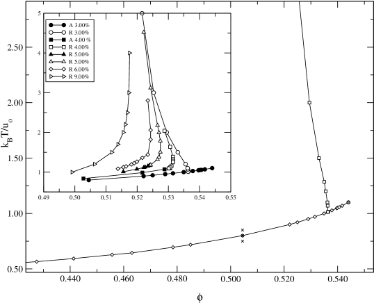
Figure 3: The phase diagram of a square-well system in the PY approximation for a square well relative width $\epsilon=0.03$. The inset shows the complete phase diagram, where the AGL and the RGL are given for various values of $\epsilon$. From [6].

(i) For high enough temperatures the repulsive glass lines, RGL, tend to converge to a value approaching the critical volume fraction for hard-sphere systems $\phi_{c}\approx 0.516$, corresponding to the fact that for large $T$ the short-range part of the inter-particle potential weakly affects the dynamics. In this case the microscopic effect described by the MCT is the excluded volume cage effect, the impossibility of the molecules to move freely due to the presence of the neighbouring particles.

(ii) On lowering the temperature a liquid stabilising effect due to the attractive forces sets in, so that the liquid-glass lines tend to extend to larger values of the volume fraction. This behaviour gives also rise to the possibility of the glass melting when lowering the temperature.

(iii) The reentrant behaviour characterises the interplay of the repulsive and the attractive inter-particle forces; the system can become a glass both when lowering or raising the temperature.

(iv) For even lower values of the temperature another phase line, the AGL, appears and it is almost parallel to the $\phi$ axis. In this case the particle motions are difficult since, due to the attractive interactions, the particle tend to form bonds.

(v) The two sections of the phase lines, RGL and AGL, intersect at a finite angle for small values of the parameter $\epsilon$. The AGL extends for higher volume fractions beyond the crossing point and finally ends in a point.

(vi) The points on the glass lines we have discussed so far all correspond to bifurcations of type $A_{2}$, while the end point of the AGL relates to a higher order bifurcation $A_{3}$.

(vii) The extension of the AGL that develops in the glass region leads to the coexistence of two different types of glasses. In order to represent the differences between the two glasses we present in figure 4 the shape of the non-ergodicity factor $f_{q}$ crossing the glass-glass transition. The results are now consistent with the experimental observation (iii) in the introduction. The width of the $f_{q}$ is related to the localisation length of the particles in the glass. If the width is larger the particles are more localised. It is evident that the colloidal particles are more localised in the attractive glass then in the repulsive one. It is also possible to show that the localisation of the length in the repulsive glass remains more or less unchanged decreasing the temperature, whereas for the attractive one the particles become more localised. This seems to confirm the idea that the repulsive glass is dominated by the so-called cage effect: when the system gets to high packing fraction the particles start to be blocked by their neighbours, at certain critical packing fraction $\phi_{c}$ each particle is trapped in a cage formed by the surrounding particles. Indeed this is a purely geometrical effect and it should not depend on temperature.

(viii) On increasing the relative square well width parameter $\epsilon$ the glass-glass line tends to shrink and finally coincides with the point of intersection of the RGL and AGL when $\epsilon\approx 0.04$. This end-point is a higher bifurcation point of type $A_{4}$. We note that there is no difference in the structure factor across this curve. Only the late stage dynamics, reflected in the values of the non-ergodicity factors, may be used to differentiate between these glasses.

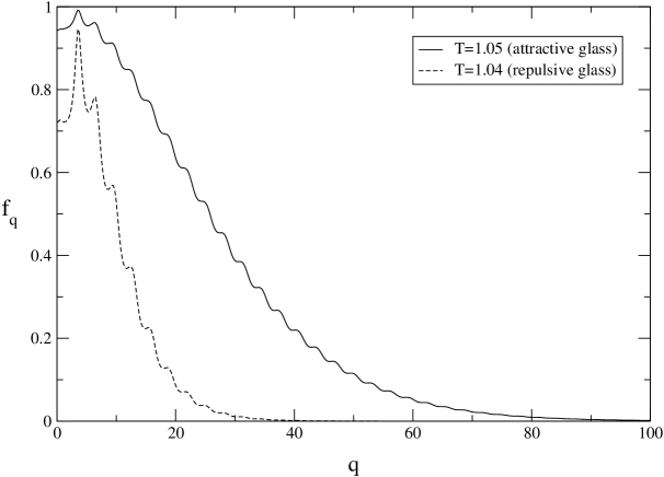
Figure 4: The typical non-ergodicity factors $f_{q}$ crossing the glass-glass transition line for $\epsilon=0.03$ and $\phi=0.544052$.

5 The intermediate scattering function

We have studied the dynamical behaviour of the system in different regions of the phase diagram, in particular in the proximity of the higher order bifurcation points $A_{3}$ and $A_{4}$. We will mainly comment on the case where the well width parameter is $\epsilon=0.03$. The wave vectors are given in units of the particles diameter. In figure 5 we present different intermediate scattering functions for $q=21.75$, obtained by solving MCT equations, approaching the glass transition at $\phi=0.504449$ and $T_{c}\simeq 0.8000$. The relevant cut across the attractive glass curve is shown in figure 3 using crosses, and a transition point. For temperatures well above the glass transition, i.e. $T=0.85$, $\phi_{q}(t)$ presents the typical liquid behaviour: after a first short-time decaying due to microscopic dynamics, the correlation function starts to relax toward ergodicity and no sign of a critical slowing down is evident. When the system becomes close enough to the transition temperature ($T=0.80010$ in figure 5) the system starts to freeze and the typical two step relaxation scenario starts to be evident. We note that we are here crossing that transition curve which we believe corresponds to the process of gelation at high density. We see, therefore, that we may expect the characteristic behaviour of a glass transition in the slow dynamics near gelation at high density.

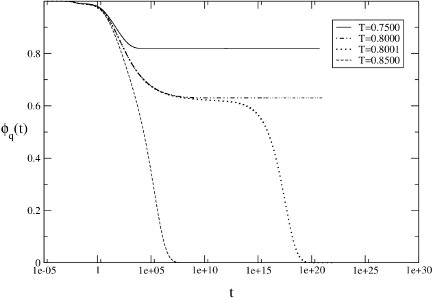
Figure 5: Time dependence of the density correlators for $q=21.75$, $\epsilon=0.03$, $\phi=0.504449$ and different temperatures.

Once the system is below the transition temperature (the case $T=0.80000$ in figure 5), $\phi_{q}(t)$ corresponding to the gel does not relax to zero anymore, the system is non-ergodic. In this situation there is only part of the $\beta$-relaxation toward a non-zero constant value, i.e. the non-ergodicity parameter $f_{q}\neq 0$. Perhaps it is useful now to discuss some of the MCT predictions for the asymptotic behaviour of the intermediate scattering function (see for example [2] and references therein). In the time region where $t_{0}\ll t\ll\tau_{\alpha}$ the so-called factorisation theorem holds

$$\phi_{q}(t)=f^{c}(q)+h_{q}G(t)$$ (17)

$t_{0}$ being a typical macroscopic time, $\tau_{\alpha}$ the $\alpha$ relaxation time scale and $f^{c}_{q}$ the critical non ergodicity parameter. Equation 17 implies a universal behaviour in which wave-vectors and time factorize. $G(t)$ is a scaling function which describes the whole relaxation pattern. Near the glass transition the behaviour of the function $G(t)$ may be calculated analytically in the proximity of the $\alpha$ and $\beta$ relaxation. It can be shown that the asymptotic behaviour can be expressed in terms of a rescaled time $\tau=t/t_{\sigma}$ where $t_{\sigma}$ is a time scale that depends crucially on the distance to the transition, i.e. on the separation parameter $\sigma$ [2]. Close to the glass transition, for $T>T_{c}$, $G(\tau)$ is given by

$$G(\tau\ll 1)\sim 1/\tau^{a}$$ (18)

$$G(\tau\gg 1)\sim-\tau^{b}$$ (19)

where the two exponents are related to the exponent parameter $\lambda$, which is obtained from a stability matrix [2], via the relation $\lambda=\Gamma^{2}(1-a)/\Gamma(1-2a)=\Gamma^{2}(1+b)/\Gamma(1+2b)$, which implies $0<a<1/2$ and $0<b<1$. The scaling behaviour of the correlation function changes in the proximity of higher bifurcation points. In particular it is possible to show that near an $A_{3}$ point $G(t)\sim 1/\ln(t/t_{1})$ whereas near an $A_{4}$ it goes like $G(t)\sim 1/\ln^{2}(t/t_{1})$, where $t_{1}$ is a microscopic time scale [26]. This is quite a remarkable behaviour and represents a rather strong prediction of the theory. There have been reports of such behaviour in some system [20, 26], and it will be interesting to see if this phenomenon is discovered in a variety of different colloidal systems.

6 Mechanical properties

Two particularly interesting quantities to investigate in the vicinity of the glass transition are the shear viscosity and the elastic shear modulus. Those two quantities can be measured in real systems and such measurements can provide a good insight in the glass transition phenomena and its relations with MCT. The complex shear viscosity $\eta^{*}(\phi,T,\omega)$ can be calculated in terms of the normalised time correlation function of the density fluctuations $\phi_{k}(t)$ [25, 26]

$$\eta^{*}(\phi,T,\omega)={{k_{B}T}\over{60~{}\pi^{2}}}{\int_{0}^{\infty}}dte^{i\omega t}{\int_{0}^{\infty}}dkk^{4}{\left[{{dlnS_{k}}\over{dk}}\phi_{k}(t)\right]}^{2}$$ (20)

and is related to the complex shear modulus $G^{*}(\phi,T,\omega)$ by

$$G^{*}(\phi,T,\omega)=i~{}\omega~{}\eta^{*}(\phi,T,\omega).$$ (21)

It is possible to take the $\omega\rightarrow 0$ limit in equation 20

$$\eta^{*}(\phi,T,\omega=0)={{k_{B}T}\over{60~{}\pi^{2}}}{\int_{0}^{\infty}}dkk^{4}{\left[{{dlnS_{k}}\over{dk}}f_{k}\right]}^{2}$$ (22)

and this gives the static shear viscosity. We note that this formula, in that it depends on the square of the correlation function, is different in structure from that used by Weitz and co-workers, where the stress-relaxation function is linearly related to the density correlation function [27]. This difference would lead, in principle, to substantially different predictions for the loss modulus, and in particular around its minimum. It seems likely that the idea the stress modulus is linear in the correlation function is more suited to visco-elastic properties dominated by large domains, and their changing surface area under shear [28], whilst the dependence on the square of the correlation function is more suited to dense fluids where the properties are dominated by loss of mobility due to caging effects.

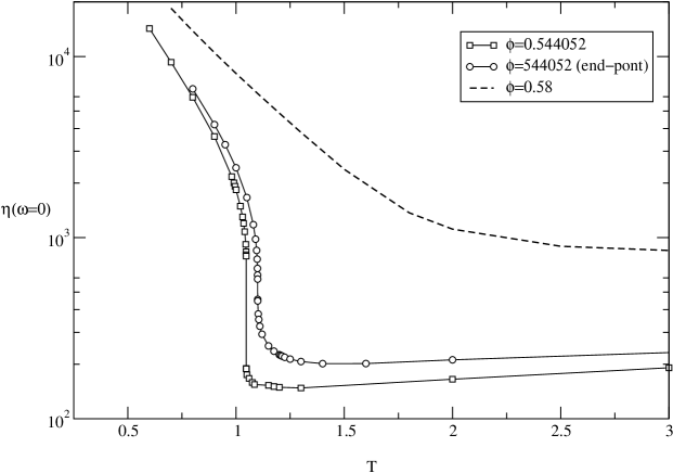
Figure 6: The static shear moduli on crossing the glass-glass transition line for $\epsilon=0.03$ and close to the $A_{3}$ bifurcation point.

All the quantities in the equations (20), (21) and (22) can be evaluated for the present system, and therefore it is possible to use the numerical solution of equation (12) in order to solve them. This has been accomplished performing the integrals with standard numerical integration over $2000$ $q$-vector varying between $0$ and $500$. In figure 6 the static shear modulus has been represented for three different packing fractions ($\phi=0.539672$, $\phi=0.544052$ and $\phi=0.580000$) as a function of the temperature. These three cases correspond to crossing the glass-glass line, crossing the $A_{3}$ point and a density where the repulsive and attractive glasses have become indistinguishable. In the first case it is clearly possible to distinguish between the two glasses. For low temperatures there is strong dependence of the elastic viscosity on the temperature, in particular the system becomes more and more rigid on decreasing the temperature. When the system crosses the glass-glass transition there is a discontinuity in the elastic response which clearly indicates that the structure is changed. Increasing further the temperature the elastic behaviour does not change so much anymore and for large temperature the system behaves like a hard spheres suspension. In this case the glass is originated by the cage effect and consequently the particle are forced to move inside a fixed volume that does not change with temperature. It is then evident how the differences between the two glasses are manifested by mechanical properties. We have noted that the difference in the shear modulus as the $A_{3}$ point is approached is described a by a power law, and it is also possible to show that in this regime the differences in mechanical properties of the two systems are due to the different shape of the non-ergodicity parameter $f_{q}$, and hence the long time residual motions in the gel, and not to the contribution of the equilibrium structure factor [29].

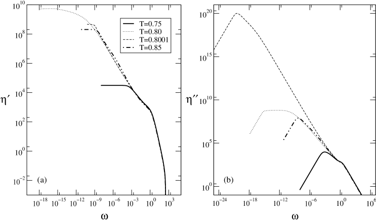
Figure 7: Relaxation of the shear viscosity on crossing the attractive transition line for $\epsilon=0.03$ and $\phi=0.504449$.

We have performed this calculation also for the dynamical quantities defined by (20) and (21). It is evident that, if the system is in the glassy phase we have for the long time behaviour of the density correlators $\phi_{q}(t\rightarrow\infty)=f_{q}\neq 0$, and consequently the integral in (20) is unbounded. Thus the solution posses a zero frequency pole. In order to obtain convergent solutions for a glass we have replaced $\phi_{q}(t)$ with $\hat{\phi}_{q}(t)=\phi_{q}(t)-f_{q}$ which decays to zero at infinite time. In figure 7a and figure 7b the real and the imaginary part of the complex viscosity, $\eta^{\prime}(\omega)$ and $\eta^{\prime\prime}(\omega)$, are presented for a fixed volume fraction, $\phi=0.504449$, for different temperatures, approaching and crossing the glass transition. In figures 8a and 8b $G^{\prime}(\omega)$ and $G^{\prime\prime}(\omega)$ are shown for the same points as figure 7. Since figures 7 and 8 contain the same information we discuss only figure 8. $G^{\prime}(\omega)$ represents the elastic response of the material: the higher its value the stiffer the material at that frequency scale. The imaginary part of the shear modulus describes the viscous behaviour of the system and so the dissipation. Both quantities can be easily measured experimentally, for example as the response of a sample to small oscillatory shears which weakly perturb the system [27]. Approaching the glass transition we note that the $G^{\prime}(\omega)$ begins to develop a shoulder at low frequency. This effect is due to the slowing down of the dynamics of the system, in other words the formation of the plateau in the $\phi_{q}(t)$ is responsible for the formation of a region where $G^{\prime}(\omega)$ varies only slightly with frequency. The range of such a region tends to increase approaching $T_{g}$. Indeed a similar behaviour has been observed experimentally in measurements of linear viscoelasticity in a colloidal suspension with hard sphere interaction [27]. If the system is in a glassy state the value of the real part of the static shear modulus $G^{\prime}(\omega=0)$ is finite, indicating that the system is solid and consequently it presents an elastic behaviour. In the liquid phase, however, the system does not show any elastic behaviour so the $G^{\prime}(\omega=0)$ tends to zero. It is then clear that at the glass transition the system abruptly changes its behaviour, presenting a singularity in the static shear modulus. In figure 8b the behaviour of the imaginary part of the shear modulus is represented. At high frequency the curves for different temperature are the same, showing the microscopic dynamics which is the same for all the temperatures. Approaching the glass transition a second maximum starts to emerge. Such a maximum represents the $\alpha$-relaxation and it moves toward low frequency on decreasing the distance to the glass transition temperature $T_{g}$. The minimum of $G^{\prime\prime}(\omega)$ corresponds to the plateau region in time, and the power law behavior in frequency on both sides has been already observed in hard spheres systems [27].

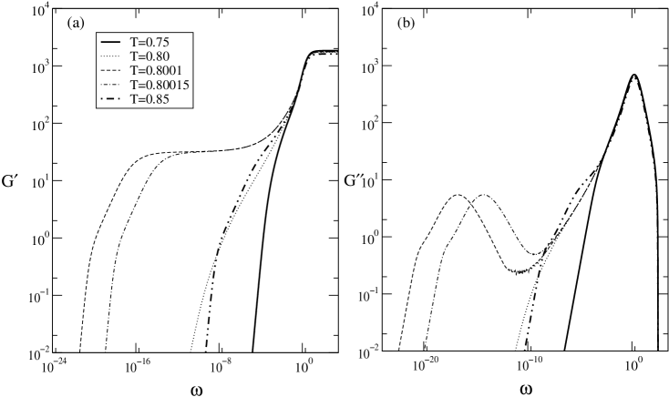
Figure 8: Relaxation of the shear modulus on crossing the attractive transition line for $\epsilon=0.03$ and $\phi=0.504449$.

7 Conclusions

In this paper we have outlined some of the experimental observations that have been made of particle gels in colloidal systems where we know there to be a strong short-ranged potential. We have shown that all of these features may be interpreted within the paradigm that such particle gels represent a new type of attractive glass. However, having made this correspondence, we then find a number of predictions of new phenomena that have yet to be confirmed experimentally, or are just being so. These include the re-entrant behaviour for the phase diagram, the logarithmic dynamic behaviour near this re-entrant regime, and in the general the characteristic alpha relaxational behaviour near gelation. We have calculated the mechanical manifestations of these phenomena also. Thus we have shown how the glass-glass transition may be studied using the shear modulus, and that the particle gel must be expected to be much stiffer than the colloidal glass, but that the differences between them vanishes near the $A_{3}$ point. We have also studied, to our knowledge for the first time, the frequency dependent modulus and loss modulus for these systems, using the paradigm that the system is undergoing a glass transition. MCT type treatments seem to be suited to study colloidal systems of this type because, at least of the repulsive system, the glass transition seems to lack some of the fluctuations of molecular liquids. We also can calculate phase diagrams, and mechanical and scattering properties from a single theory. We expect that, in future, dense particle gels will be better fitted to the theory present here, than previous phenomenological treatments.

There remains much to be done in many directions. It now begins to seems likely that the glass paradigm is suitable for interpretation of particle gelation. However we must await further detailed experimental work to see just how extensive the agreement with MCT type treatments will be. We may also speculate that this type of idea will have much broader significance that particle gels. There is every reason to hope that polymer gelation and protein gelation may also find a description in similar terms. Certainly this is a rich area for future exploration.

References

References

- [1] Pusey P N 1991 Liquids, Freezing and Glass Transition edited by Hansen J -P, Levesque D, and Zinn-Justin J (Amsterdan: North-Holland) p 763
- [2] Götze W 1991 Liquids, Freezing and Glass Transition edited by Hansen J -P, Levesque D, and Zinn-Justin J (Amsterdan: North-Holland) p 287
- [3] van Megen M and Pusey P N 1991 Phys. Rev. A 43 5429
- [4] Poon W C K, Selfe J S, Robertson M B, Ilett S M, Pirie A D, and Pusey P N 1992 J. Phys. II France 3, 1075
- [5] Fabbian L, Götze W, Sciortino S, Tartaglia P, and Thiery F 1999 Phys. Rev. E 59 R1347 —–1999 Phys. Rev. E 60 2430
- [6] Dawson K, Foffi G, Fuchs M, Götze W, Sciortino F, Sperl M, Tartaglia P, Voigtmann Th, Zaccarelli E 2000 Phys. Rev. E 63 1140
- [7] Götze W 1999 J. Phys.: Condens. Matter 11 A1
- [8] van Megen M 1995 Transp. Theory Stat. Phys. 24 1017
- [9] Kob W and Andersen H C 1995 Phys. Rev. E 51, 4626 —–1995 Phys. Rev. E 52, 4134
- [10] Gallo P, Sciortino F, Tartaglia P, Chen S -H 1996 Phys. Rev. Lett. 76 2730
- [11] Rinaldi A, Sciortino F, Tartaglia P 2001 Phys. Rev. E in press
- [12] Sciortino F, Kob W 1999 Phys. Rev. Lett. 86 648
- [13] Verduin H and Dhont J K G 1995 J. Colloid Interface Sci. 172 425
- [14] Lobry L, Micali N, Mallamace F, Liao C, and Chen S -H 1999 Phys. Rev. E 60 7076
- [15] Kranendonk W G T and Frenkel D 1988 Mol. Phys. 64 403
- [16] Meller A, Gisler T, Weitz D A, and Stavans J 1999 Langmuir 15 1918
- [17] Grant M C and Russel W B 1993 Phys. Rev. E 47 2606
- [18] Rueb C J and Zukoski C F 1997 J. Rheology 41 197
- [19] Rueb C J and Zukoski C F 1998 J. Rheology 42 1451
- [20] Mallamace F, Gambadauro P, Micali N, Tartaglia P, Liao C, Chen S -H 2000 Phys. Rev. Lett. 84 5431
- [21] Hansen J P and McDonald I R 1986 Theory of Simple Liquids (London: Academic Press)
- [22] Baxter R J 1968 Aust. J. Phys. 21 563
- [23] Bergenholtz J and Fuchs M 1999 Phys. Rev. E 59 5706
- [24] Dawson K, Foffi G, McCullagh G, Zaccarelli E, Sciortino F, Tartaglia P 2001 unpublished
- [25] Bengtzelius U, Götze W, Sjölander A 1984 J. Phys. C: Solid State Phys. 17 5915
- [26] Sjögren L 1991 J. Phys.: Condens. Matter 3 5023
- [27] Weitz D A 1995 Phys. Rev.Lett. 75, 2770
- [28] Onuki, A 1987 Phys. Rev. A 35, 5149
- [29] Zaccarelli E, Foffi G, Dawson K A, Sciortino F and Tartaglia P 2001 Phys. Rev. E 63, 31501