Analysis of the $\infty$-replica symmetry breaking solution of the Sherrington-Kirkpatrick model

Abstract

In this work we analyse the Parisi’s $\infty$-replica symmetry breaking solution of the Sherrington - Kirkpatrick model without external field using high order perturbative expansions. The predictions are compared with those obtained from the numerical solution of the $\infty$-replica symmetry breaking equations which are solved using a new pseudo-spectral code which allows for very accurate results. With this methods we are able to get more insight into the analytical properties of the solutions. We are also able to determine numerically the end-point $x_{\rm max}$ of the plateau of $q(x)$ and find that $\lim_{T\to 0}x_{\rm max}(T)>0.5$.

I Introduction

Since its proposal in the 80’s the behaviour of the Parisi $\infty$-replica symmetry breaking ($\infty$-RSB) solution of the Sherrington-Kirkpatrick model has been extensively investigated both qualitatively and quantitatively MPV ; FH . Despite this enormous amount of work, which has revealed many of the properties of the solutions, a complete control of the solution is still missing. One of the reasons can be traced back to the fact that till now only low order expansions were used, moreover applied often to reduced forms $\infty$-replica symmetry breaking equations valid only near the critical temperature. From the numerical point of view there are only few works which confirm the general properties of the solution but do not allow for high accuracy. On the other hand $\infty$-replica symmetry breaking solutions of the type encountered in the SK model have been found in other models of interest in different fields, e.g., in computer science with solvability problems Luca or in the study of the structural glass transition G85 ; KT87 ; SNA97 .

Motivated by these problems we believe that it would be quite useful to have some reliable and efficient tool to find good approximations of the full solution also far from the critical points. In this work we reconsider two approaches. The first one is based on expansions for temperatures near the critical temperature $T_{c}$. As said above previous works considered only low order expansions P7980 ; K83 ; S85 . Here, by using algebraic manipulators, we push the expansion to rather high orders and resumming it via Padè resummation technique we are able to a have good estimate of the solution for a wide range of temperature below $T_{c}$.

The second approach is numerical. Previous numerical studies of the $\infty$-replica symmetry breaking solution used a naive integration scheme based on the direct discretization of the Parisi’s equation VTP81 ; SDJPC84 ; topomoto ; B90 . The main disadvantages of this approach are the large amount of memory needed for a good resolution of the solution and the numerical problems arising when $\dot{q}(x)$ is small. To overcome these problems we developed a new numerical scheme based on a pseudo-spectral algorithm which allows for rather accurate results for all temperatures with a reasonable amount of memory. Moreover the use of pseudo-spectral methods makes the whole code rather fast.

We stress that while the methods we are going to discuss are applied here to the Sherrington - Kirkpatrick model, they have a wider range of application. In principle can be applied to any model with $\infty$-replica symmetry breaking type solution Luca .

We find that for the Sherrington - Kirkpatrick model the Parisi solution $q(x)$ is not an odd function as one may expect from its physical meaning. At any $T<T_{c}$, the Taylor expansion of $q(x)$ in powers of $x$ contains both odd as well as even powers of $x$. The only term which is missing is $x^{2}$. The presence of the fourth oder derivative was first noted by Temesvari Temes . Often, instead of $q(x)$, it is more useful to consider the overlap probability distribution function $P(q)$, which gives the probability of finding two states with mutual overlap $q$ according to the Gibbs measure. The two quantities are related by DY83 ; P83 :

$$P(q)=\frac{dx}{dq}$$ (1)

where $x(q)$ is the inverse function of $q(x)$. In the absence of external magnetic fields the function $P(q)$ must be an even function of $q$. The computed function $q(x)$ is however defined only for positive values, therefore it determines only the right branch of the function $P(q)$. If we define $\tilde{P}(q)=dx/dq$ for $q>0$ then full $P(q)$ is given by the symmetrized expression

$$P(q)=\frac{1}{2}\tilde{P}(-q)+\frac{1}{2}\tilde{P}(q)$$ (2)

It is easy to see that the presence of non-zero even derivatives of $q(x)$ at $x=0$ makes the function $P(q)$ non analytical at $q=0$:

$$P(q)=c_{0}+c_{2}q^{2}+c_{3}|q|^{3}+\ldots$$ (3)

so that $P(q)$ has discontinuous derivatives at $q=0$.

We shall discuss two different methods of computing the expansions. The first, discussed in Section II, performs expansion before imposing stationarity of the free energy functional. The two steps however can be inverted, i.e., the expansion can be done after stationarity is imposed, Section III. The two approaches are obviously equivalent and the advantage of using one or the other only depends on which quantity one is interested in. Since the expansions are likely to be asymptotic some resummation scheme, such as Padè discussed in Section IV, are needed. Finally in Section V we present a new integration procedure and compare the analytical results with those obtained from a direct numerical solution of the $\infty$-replica symmetry breaking equations.

II Expansion of the free energy functional

The Parisi’s free energy $f$ for a the SK model in an external field $h$ at temperature $T$ is P80 :

$$-f=\frac{\beta}{4}\,\Bigl{(}1-2\,q(1)+\int_{0}^{1}dx\,q^{2}(x)\Bigr{)}+\int_{-\infty}^{+\infty}\frac{dy}{\sqrt{2\pi q(0)}}\exp\left(-\frac{(y-h)^{2}}{2\,q(0)}\right)\phi(0,y)$$ (4)

where $\phi(0,y)$ is the solution evaluated at $x=0$ of the the Parisi’s equation

$$\dot{\phi}(x,y)=-\frac{\dot{q}(x)}{2}\,\Bigl{[}\phi^{\prime\prime}(x,y)+\beta\,x\,\phi^{\prime}(x,y)^{2}\Bigr{]}$$ (5)

with the boundary condition

$$\phi(1,y)=\beta^{-1}\log\left(2\cosh\beta y\right)$$ (6)

where we have used the standard notation and denote derivatives with respect to $x$ by a dot and derivatives with respect to $y$ by a prime. The order parameter $q(x)$ at temperature $T$ is obtained by the stationarity condition of (4) with respect to variations of $q(x)$, while the value of (4) at the stationarity point gives the free energy $f(T)$.

To expand the free energy functional (4) in powers of $\tau=T_{c}-T=1-T$ we observe that in the absence of external fields $q(x)$ is different from $q(1)$ only in a region $[0,x_{\rm max}]$ with $x_{max}=O(\tau)$ P7980 , so that an expansion in power of $\tau$ must correspond to an expansion of the same order in $x$. Therefore to compute the free energy to order $n$ we insert into eq. (4) the following expansions:

$$q(1)=\sum_{i=1}^{n-2}\,a_{i}\,\tau^{i}$$ (7)

and

$$x(q)=\sum_{i=1}^{n-3}\,\sum_{j=0}^{n-3-i}b_{ij}\,q^{i}\,\tau^{j}.$$ (8)

The coefficients of the expansion of the function $\phi(q,y)$ about $q=q(1)$ and $y=0$ can be obtained by repeated differentiation with respect to $q$ of the equation

$$\frac{\partial\phi}{\partial q}=-\frac{1}{2}\left[\frac{\partial^{2}\phi}{\partial y^{2}}+x(q)\left(\frac{\partial\phi}{\partial y}\right)^{2}\right].$$ (9)

Differentiating $j$ times with respect to $y$ this equation, mixed derivatives $\phi^{(1,j)}(q,y)$ can be eliminated in favor of derivatives with respect to $y$ only. In the absence of an external magnetic field the last term in equation (4) reduces to $\phi(0,0)$ greatly simplifying the calculation since at each step we can eliminate all terms containing odd derivatives of $\phi$ with respect to $y$, as for example $(\partial\phi/\partial y)^{2}$ in the previous equation, since all these vanish if evaluated at $y=0$ being $\phi(q,y)$ and even function of $y$.

Collecting all terms with the same power of $\tau$ the free energy functional (4) is written as

$$f=\sum_{i=0}^{n}\,c_{i}[\{a\},\{b\}]\,\tau^{i}.$$ (10)

This expression must be stationary with respect to variations of $a$’s and $b$’s for any $\tau$. Imposing stationarity of each $c_{i}$ we can find the value of the parameters $a$ and $b$. For example to order $\tau^{6}$ we have:

$$q(x)=\left(\frac{1}{2}+\frac{3}{2}\,\tau+2\,\tau^{3}-9\,\tau^{4}+\frac{336}{5}\,\tau^{5}\right)\,x + \left(-\frac{1}{8}+\frac{25}{8}\,\tau+3\,\tau^{2}+38\,\tau^{3}\right)\,x^{3}$$ (11)

$$+ \left(-1-9\,\tau-30\,\tau^{2}\right)\,x^{4}+\left(\frac{351}{320}+\frac{9189}{320}\,\tau\right)\,x^{5}-\frac{27}{5}\,x^{6}$$

and

$$x_{\rm max}=2\,\tau-4\,\tau^{2}+12\,\tau^{3}-69\,\tau^{4}+\frac{2493}{5}\,\tau^{5}-\frac{20544}{5}\,\tau^{6}.$$ (12)

By using this procedure we have obtained the free energy up to order $30$, $q(x)$ to order $13$ and $q(1)$ to order $14$ because despite the fact that the free energy is evaluated to order $n$, the variational relations allow to determine $x(q)$ only to order $[(n-3)/2]$ and $q(1)$ only to order $[(n-1)/2]$.

From eq. (11) we clearly see that $q(x)$ contains even powers of $x$, with the exclusion of $x^{2}$. In the next Section we shall derive exact relations among the derivatives of $q(x)$ at $x=0$ from which follow that $q^{(2)}(x=0)=0$ but $q^{(4)}(x=0)\not=0$.

III Expansion of the order parameter $q(x)$

To evaluate the derivatives of the order parameter $q(x)$ at $x=0$ we use a variational approach developed by Sommers and DupontSDJPC84 . This method as also the advantage of leading to exact relations among derivatives of different order, so can be used to test the findings of the previous Section in a non-perturbative way. The starting point is the variational form of the Parisi’s free energy $f$:

$$-f = \frac{\beta}{4}\,\Bigl{(}1-2\,q(1)+\int_{0}^{1}dx\,q^{2}(x)\Bigr{)}+\int_{-\infty}^{+\infty}\frac{dy}{\sqrt{2\pi q(0)}}\exp\left(-\frac{(y-h)^{2}}{2\,q(0)}\right)\phi(0,y)$$ (13)

$$- \int_{-\infty}^{+\infty}dy\ P(1,y)\,\bigl{[}\phi(1,y)-T\log\left(2\cosh\beta y\right)\bigr{]}$$

$$+ \int_{0}^{1}dx\int_{-\infty}^{+\infty}dy\ P(x,y)\left[\dot{\phi}(x,y)+\frac{\dot{q}(x)}{2}\,\Bigl{[}\phi^{\prime\prime}(x,y)+\beta\,x\,\phi^{\prime}(x,y)^{2}\Bigr{]}\right].$$

Imposing stationarity with respect to variations of $P(x,y)$, $P(1,y)$, $\phi(x,y)$, $\phi(0,y)$ and $q(x)$, one obtains the variational equations:

$$q(x)=\int dy\,P(x,y)\,m^{2}(x,y)$$ (14)

$$\dot{m}(x,y)=-\frac{\dot{q}(x)}{2}\,\Bigl{[}m^{\prime\prime}(x,y)+2\,\beta\,x\,m(x,y)\ m^{\prime}(x,y)\Bigr{]}$$ (15)

$$\dot{P}(x,y)=\frac{\dot{q}(x)}{2}\Bigl{[}P^{\prime\prime}(x,y)-2\,\beta\,x\,[m(x,y)\,P(x,y)]^{\prime}\Bigr{]}$$ (16)

with initial conditions (in the absence of a magnetic field)

$$m(1,y) = \tanh(y/T)$$ (17)

$$P(0,y) = \delta(y)$$ (18)

These equations are the starting point of both the expansion discussed in this Section and the numerical solution.

A time scale $\tau_{x}$ can be associated to the order parameter $q(x)$ such that for times of order $\tau_{x}$ states with an overlap equal to $q(x)$ or greater can be reached by the system. In this picture the $P(x,y)$ and $m(x,y)$ become respectively the probability distribution of frozen local fields $y$ and the local magnetization in a local field $y$ at the time scale labeled by $x$ SDJPC84 ; MPV .

The derivatives of $q(x)$ can be obtained by successive $x$-derivation of eq. (14). The procedure is simplified by the use of the following identity S85 :

$$\frac{d}{dx}\int dy\,P(x,y)\,f(x,y)=\int dy\,P(x,y)\,\Omega(x,y)\,f(x,y)$$ (19)

where

$$\Omega(x,y)=\frac{\partial}{\partial x}+\frac{\dot{q}}{2}\left(\frac{\partial^{2}}{\partial y^{2}}+2\,\beta\,x\,m(x,y)\frac{\partial}{\partial y}\right)$$ (20)

The application of the operator $\Omega(x,y)$ generates derivatives of the function $m(x,y)$ with respect to $x$ and $y$. Mixed derivatives such as $m^{(1,j)}(x,y)$ can be eliminated in favor of derivatives of $m(x,y)$ respect only to $y$ by deriving equation (15) $j$ times with respect to $y$.

The first application of this procedure yields

$$\dot{q}(x)=\dot{q}(x)\,\int dyP(x,y)(m^{\prime})^{2}$$ (21)

which for $\dot{q}(x)\neq 0$ simply reads

$$1=\int dy\,P(x,y)\,m^{\prime}(x,y)^{2}.$$ (22)

The procedure can be iterated infinitely. For example, the next three applications leads respectively to

$$0=-\frac{2x}{T}\int dyP(m^{\prime})^{3}+\int dyP(m^{\prime\prime})^{2}$$ (23)

$$\frac{2}{T}\int dyP(m^{\prime})^{3}=\dot{q}\int Pdy\left((m^{\prime\prime\prime})^{2}-\frac{12x}{T}m^{\prime}(m^{\prime\prime})^{2}+6\left(\frac{x}{T}\right)^{2}(m^{\prime})^{4}\right)$$ (24)

and

$$\int Pdy\left(\frac{(18x\dot{q}+6x^{2}\ddot{q})(m^{\prime})^{4}}{T^{2}}-\frac{(18\dot{q}T+12x\ddot{q}T-120m^{\prime}x^{2}\dot{q}^{2})m^{\prime}(m^{\prime\prime})^{2}}{T^{2}}\right.$$

$$\left.+\frac{-30x\dot{q}^{2}(m^{\prime\prime})^{2}+\ddot{q}m^{\prime\prime\prime}T-20x\dot{q}^{2}m^{\prime}(m^{\prime\prime\prime})}{T}m^{\prime\prime\prime}-\frac{24x^{3}\dot{q}^{2}(m^{\prime})^{5}}{T^{3}}+\dot{q}^{2}(m^{\prime\prime\prime\prime})^{2}\right)=0$$ (25)

We are interested into the derivatives of $q(x)$ at $x=0$, so we take the limit $x\rightarrow 0$ of the above equations. The limit can be done in trivial way and, since the function $P(0,y)$ reduce to a $\delta$-function [see eq. (18)], the equations are greatly simplified. Moreover since $m(x,y)$ is an odd function of $y$ for any $x$ clearly $m^{(0,j)}(0,0)=0$ for any even $j$. In this limit equations (22), (24) and (25) reduce respectively to:

$$1 = m^{\prime}(0,0)$$ (26)

$$\frac{2}{T}m^{\prime}(0,0)^{3} = \dot{q}(0)m^{\prime\prime\prime}(0,0)^{2}$$ (27)

$$\ddot{q}(0)m^{\prime\prime\prime}(0,0)^{2} = 0$$ (28)

while equations (14) and (23) become trivial identities.

From equations (26) and (27) we have

$$m^{\prime\prime\prime}(0,0)=-\sqrt{\frac{2}{T\dot{q}(0)}}\neq 0$$ (29)

therefore (28) implies that $\ddot{q}(0)=0$ as already found in Ref. S85 .

To obtain information on the fourth derivative of $q(x)$ the above procedure must be iterated two more times. Since successive derivatives yields expressions with a rapidly growing number of terms we only report the limit $x\rightarrow 0$ result:

$$\frac{18\dot{q}(0)}{T^{2}}+q^{(3)}(0)m^{\prime\prime\prime}(0,0)^{2}-\frac{38\dot{q}(0)^{2}m^{\prime\prime\prime}(0,0)^{2}}{T}+\dot{q}(0)^{3}m^{(0,5)}(0,0)=0$$ (30)

$$q^{(4)}(0)m^{\prime\prime\prime}(0,0)-\frac{96\dot{q}(0)m^{\prime\prime\prime}(0,0)^{3}}{T}=0$$ (31)

where equation (26) and the exact result $\ddot{q}(0)=0$ have been used. Note that equation (31), with equation (29), gives a complete determination of the quartic derivative of $q(x)$ at $x=0$ as a function of the temperature $T$ and of the first derivative $\dot{q}(x=0)$:

$$q^{(4)}(0)=-\frac{96\sqrt{2}\dot{q}(0)^{5/2}}{T^{3/2}}$$ (32)

This relation shows that the function $q(x)$ does not have a well defined parity Temes .

Going to higher orders one can show that all the even derivatives can be expressed in terms of the odd ones; for instance we have

$$q^{(6)}(0)=-\frac{34272\sqrt{2}\dot{q}(0)^{7/2}}{T^{5/2}}-\frac{1056\sqrt{2}\dot{q}(0)^{3/2}q^{(3)}(0)}{T^{3/2}}$$ (33)

and so on.

In the limit $T\to 0$ we have $T\,\dot{q}(0)=0.743\pm 0.002$. Note that if we take $\dot{q}(0)\sim 1/T$ for $T\to 0$ the previous equations implies that all the derivatives diverge with the temperature as $q^{(n)}(0)\sim 1/T^{n}$, in agreement with the Parisi-Toulouse scaling $q(x,T)=q(\beta x)$ VTP81 ; PT80 . Note that we have derived this scaling under strong hypothesis that it must be valid asymptotically for $T\to 0$ and $\beta x\to 0$.

This approach also provides an alternative method to compute the expansion of $q(x)$ in powers of $x$ and $\tau$: starting from $q(x)$ evaluated at a given order in $x$ and $\tau$ we can compute $m^{(0,j)}(0,0)$ through (15) and then $q(x)$ at the next order through the set of equations (26),(28), (30),(31) and so on. The set of equations can be solved iteratively. By this method we were able to compute the series expansion of $q(x)$ up to order $20$, improving the results of previous section.

IV Resummation of the expansions

Unfortunately all the expansions derived in the previous Sections are likely to be asymptotic and to obtain sensible estimates of the various quantities of interest some form of resummation must be done. Here we shall consider the standard Padè approximants which for a series of degree $N+M$ reads BO78 :

$$P^{N}_{M}(x)=\frac{\sum_{i=0}^{N}\,a_{i}\,x^{i}}{1+\sum_{i=1}^{M}\,b_{i}\,x^{i}}$$ (34)

where the coefficients are chosen so that the first $(N+M+1)$ terms of the Taylor expansion of $P^{N}_{M}(x)$ match the the first $(N+M+1)$ terms of the of the original series. In the following we shall call this the Padè approximant $(N,M)$.

The first problem we faced is that despite the fact that the series have alternate signs, they are not Stijlties integral and therefore we cannot obtain in a systematic way a sequence of lower and upper bounds BO78 . This difficulty can be overcome by noticing that most of the quantities we are interested in, such as for example free energy or entropy or $q(1)$, do have a null derivative at $T=0$. Therefore an indication on the quality of the approximants can be obtained by analyzing the behaviour near $T=0$. For example, the free energy as a function of $T$ is reproduced quite well by many Padè approximants, even at very low orders, however some of these have a positive derivative at $T=0$ while others negative, see Fig. 1. By inspecting the figure we can safely assume that approximants with positive derivative give an upper bound, while those with negative derivative a lower bound, for the true free energy Note .

Figure 1: Free energy as function of $\tau=1-T$ for different Padè approximants. Top to bottom: $(14,16)$, $(13,12)$, $(12,11)$, $(10,11)$ and $(17,10)$.

As a general fact we obtain that the best Padè approximants at a given order in $\tau$ are those with nearly the same degree of the numerator and the denominator. We stress, however, that as usual with asymptotic expansion an increase of the order in $\tau$ does not necessarily correspond to an improvement of the precision. With this procedure we obtain for the free energy an estimate with at least $16$ digits precision at $T=0.9$ and $8$ digits at $T=0.5$, and for the ground state energy $E_{0}=-.76321\pm.00003$ in agreement with Parisi’s estimate $E_{0}=-.7633\pm.0001$ P80 . A similar analysis can be used to determine the value of $x_{\rm max}$ as a function of temperature, the result is shown in Fig. 2. The value of the breaking point is finite in the limit $T\rightarrow 0$

$$x_{max}(0)=.548\pm.005,$$ (35)

see inset Figure 2, and slightly larger than the value $1/2$ predicted by the Parisi-Toulouse scaling, in agreement with the approximate nature of this relation VTP81 ; PT80 .

Figure 2: $x_{\rm max}$ as function of $\tau=1-T$. Inset: $x_{\rm max}$ as function of $\tau=1-T$ with different Padè approximats. From top to bottom $(7,10)$, $(9,9)$, $(8,12)$, $(6,7)$ and $(7,8)$.

The analysis of the function $q(x,T)$ is more complex, because not only the Taylor expansion of $q(x)$ in powers of $x$ around any $0<x<x_{max}$ is likely to be asymptotic for any fixed temperature, but the expansion in $\tau$ of the coefficients of the $x$-expansion are themselves non convergent. Therefore one should use a double Padè expansion, one for the coefficients and one for $q(x)$. The procedure however is quite difficult because we do not have a systematic way of choosing the best approximant and, moreover, coefficients of higher order are known with less precision in $\tau$. A better approach is to construct the function $q(x)$ directly point by point by computing $q(mx_{\rm max})$ where $m=i/n$, $(i=0,1,\ldots\,n)$ for fixed $n$. For any $m$ and $T$ the quantity $q(mx_{\rm max})$ is itself a power series in $\tau$ which can be summed up using Padè approximants. With this procedure the function $q(x)$ can be determined for different $x$-resolution just changing the value of $n$, e.g., $n=50,100,1000$, and using the value of $x_{\rm max}$ previously found, see Fig. 2. In Figure 3 the function $q(x)$ is shown for various temperatures $T$.

Figure 3: $q(x)$ as function of $x$ for various temperatures. From bottom to top $T=0.95$ to $T=0.30$ in step of $0.05$.

This method can be extended to any function of $x$ or $q$, for example, we computed the overlap probability function $P(mq_{\rm max})$ in a wide range of temperature $T>0.3$, see Figure 4. We found that the best Padè approximant is given by the $(12,7)$. By using the relation (1) we can have an independent estimation of $q(x)$ with which to test the precision of our results. By using a norm $d_{\infty}(q,q^{\prime})=\max_{0\leq x\leq 1}|q(x)-q^{\prime}(x)|$ and expansions up to order $20$ we find, for example, that $d_{\infty}(q,q^{\prime})=O(10^{-5})$ for $T=0.6$ and $d_{\infty}(q,q^{\prime})=O(10^{-4})$ for $T=0.4$.

Figure 4: $P(q)$ as function of $q$ for various temperatures. From left to right $T=0.95$ to $T=0.30$ in step of $0.05$. The data are obtained with a $(12,7)$ approximant. Note that $P(q)$ attains its minimum value for $q>0$. This happens for any temperature $T<0.961938...$.

The form of the function $q(x)$ confirms the prediction of Ref. VTP81 obtained from interpolation of the $11$-RSB solution. In particular it confirms the approximate scaling $q(x,T)\sim q(x/T)$ at low temperatures, see Figure 5. Note that the scaling fails when $\beta x\sim O(1)$, in agreement with the findings of previous section.

Figure 5: $q$ as a function of $\beta x$ for different values of $T$. Top to bottom $T=0.30$, $T=0.35$, $T=0.40$, $T=0.45$ and $T=0.50$.

Finally we mention that an alternative resummation technique based on the Borel transform give results consistent with those obtained with the Padè approximants.

V Numerical Integration of the $\infty$-RSB equations

To check the analytical results of the previous sections we have solved numerically the $\infty$-RSB equations (14) - (18) on a discrete set of points in the infinite strip $[0\leq x\leq 1$; $-\infty<y<\infty]$ and determined $q(x)$, $P(x,y)$ and $m(x,y)$. The numerical method is based on the iterative procedure of Ref. topomoto : from an initial guess of $q(x)$ the fields $m(x,y)$, $P(x,y)$ and the associated $q(x)$ are computed in order as:

1. Compute $m(x,y)$ integrating from $x=x_{0}$ to $x=0$ eqs. (15) with initial condition (17).

2. Compute $P(x,y)$ integrating from $x=0$ to $x=x_{0}$ eqs. (16) with initial condition (18).

3. Compute $q(x)$ using eq. (14).

where $x_{0}\leq 1$ (See later). The steps $1.\,\to\,2.\,\to\,3.$ are repeated until a reasonable convergence is reached, typically mean square error on $q$, $P$ and $m$ of the order $O(10^{-6})$.

The core of the numerical scheme is the integration of the partial differential equations (15) and (16) along the $x$ direction which, at difference with previous numerical studies topomoto ; B90 , is done in the Fourier Space of the $y$ variables where the equations take the form:

$$\frac{\partial}{\partial x}\,m(x,k)=\frac{k^{2}\dot{q}(x)}{2}\,m(x,k)-\frac{\beta\dot{q}(x)}{2}\,\mbox{i}k\,{\cal FT}\left[m^{2}\right](x,k)$$ (36)

and

$$\frac{\partial}{\partial x}\,P(x,k)=-\frac{k^{2}\dot{q}(x)}{2}\,P(x,k)-\beta\dot{q}(x)\,\mbox{i}k\,{\cal FT}\left[P\,m\right](x,k)$$ (37)

For each wave-vector $k$ these are ordinary differential equations which can be integrated using standard methods. To avoid the time consuming calculation of the convolutions in the non-linear term we use a pseudo-spectralOrsz code on a grid mesh of $N_{x}\,\times\,N_{y}$ points, which covers the $x$-interval $[0,x_{0}]$ and the $y$-interval $[-y_{\rm max},y_{\rm max}]$. The truncation of wave-number may introduce anisotropic effects for large $k$, therefore to ensure a better isotropy of numerical treatment we perform de-aliasing via a $N_{y}/2$ truncation deal . Finally the $x$ integration has been performed using an third-order Adam-Bashfort scheme which has the advantage of reducing the number of Fast Fourier calls AB . Typical values used are $N_{x}=100\div 5000$, $N_{y}=512\div 4096$ and $y_{\rm max}=12\div 48$. The difference between the values used for $N_{x}$ and $N_{y}$ follows from the observation that if the solution in the $y$-direction is smooth enough, then only few low wave-vectors are exited. The value of the parameter $y_{\rm max}$ fixes the $y$-range where the solution is assumed different form zero, since in the numerical algorithm is implicitly assumed that

$$P(x,y)\equiv m(x,y)=0\qquad|y|>y_{\rm max}.$$ (38)

This explain the rather large value used. The number of iterations necessary to reach a mean square error on $q$, $P$ and $m$ of order $O(10^{-6})$ depends on the initial guess of $q(x)$ but it is typically of few hundreds.

Figure 6: $q(x)$ as function of x (panel a) and $P(q)$ as function of x (panel b) at $T=0.6$ for (a: bottom to top, b: left to right) $N_{x}=50$, $N_{x}=500$, $N_{x}=1000$ and $N_{x}=5000$. In all cases $x_{0}=1$, $y_{\rm max}=48$ and $N_{y}=4096$. The dash line is the result from the perturbative solution discussed in the previous sections. Inset panel a: enlargement of the region near $x_{\rm max}$.

In Figure 6 are shown the order parameter $q(x)$ and the overlap probability distribution function $P(q)$ at $T=0.6$ computed for increasing $x$-resolution and $x_{0}=1$. As expected the agreement between the numerical and the perturbative solutions increases with the number of $N_{x}$ of $x$-grid points. However, the convergence is not uniform: it is rather fast far from $x_{\rm max}$ and much slower for $x\simeq x_{\rm max}$, see the inset of Figure 6 panel (a). This is not unexpected because for $x=x_{\rm max}$ the derivative of the order parameter $q^{(1)}(x)$ has a cusp:

$$\lim_{x\to x_{\rm max}^{-}}q^{(1)}(x)>0,\qquad\lim_{x\to x_{\rm max}^{+}}q^{(1)}(x)=0$$ (39)

making the convergence more difficult. We recall that in deriving equations (15) and (16) differentiability of $q(x)$ was assumed. The use of lower order integration schemes, as second-order Adam-Bashfort or Euler schemes, does not give sensible improvements.

Larger values of $N_{x}$ requires larger needs of computer memory therefore to increase the precision we adopted a different approach. Since $\dot{q}(x)=0$ for $x>x_{\rm max}$ equations (15) and (16) are trivial in this range and we can reduce the upper bound of the $x$-integration from $x=1$ to $x=x_{0}=x_{\rm max}$. This obviously requires the knowledge of $x_{\rm max}$ for the given temperature. However if we assume no a priori knowledge of $x_{\rm max}$ we must proceeds for successive approximations: we start from $x_{0}=1$ an then reducing it until we ‘hit’ the value of $x_{\rm max}$. This procedure is simplified by the fact that if $x_{0}<x_{\rm max}$ the shape of $q(x)$ near $x_{0}$ changes dramatically with the concavity passing from negative values for $x_{0}>x_{\rm max}$ to positive values for $x_{0}<x_{\rm max}$. In Figure 7 panel (a) are shown $q(x)$ (panel a) and $P(q)$ (panel b) at $T=0.6$ for different values of $x_{0}$, the improvement in rather evident. As additional check we have considered the equality

$$1-\int_{0}^{1}dx\,q(x)=T$$ (40)

which is satisfied by our numerical solution for all studied temperatures with at least four digits. For example we for $T=0.8$ we get $0.79999(4)$, while for $T=0.5$ the value is $0.49999(3)$.

Figure 7: Panel a: $q(x)$ for $T=0.6$ near $x_{\rm max}$ for different $x_{0}$. Panel b: $P(q)$ for $T=0.6$ for different $x_{0}$ . In all cases $N_{x}=500$, $y_{\rm max}=48$ and $N_{y}=4096$. The dash line is the result from the perturbative solution discussed in the previous sections.

Note that not only by fine tuning of $x_{0}$ we can have a good solution for $q(x)$ at the given temperature, but we also have the value of $x_{0}$. This is best seen by analyzing the concavity of $q(x)$ near $x_{0}$. In Figure 8 we show the second derivative of $q(x)$ near $x_{0}$ for $T=0.4$ and $N_{x}=500$, from which one may conclude that $0.505<x_{\rm max}<0.510$.

Figure 8: Second derivative of $q(x)$ for $T=0.4$ for different $x_{0}$ and $N_{x}=500$, $y_{\rm max}=48$ and $N_{y}=4096$.

A careful analysis of the stability of this results as function of $N_{x}$, see Figure 9, reveals, however, that the correct estimation is $0.510<x_{\rm max}<0.515$, in rather good agreement with the analytical result $x_{\rm max}=0.5111\pm 0.0002$. The same analysis for $T=0.6$ leads to $0.438<x_{\rm max}<0.440$.

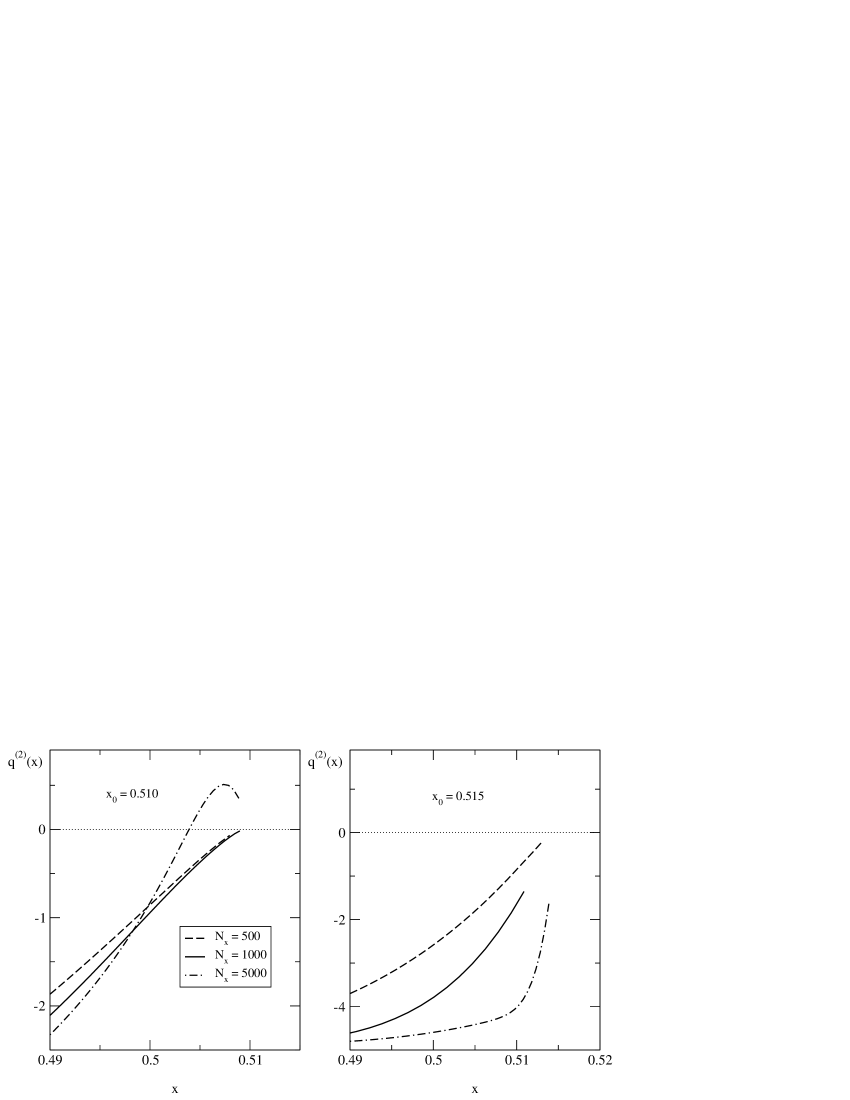
Figure 9: Second derivative of $q(x)$ for $T=0.4$ for different $N_{x}$ and $x_{0}=0.510$, $y_{\rm max}=48$ and $N_{y}=4096$. Left panel: $x_{0}=0.510$, increasing $N_{x}$ leads to a positive value of $q^{(2)}(x_{0})$ implying $x_{0}=0.510<x_{\rm max}$. Right panel: $x_{0}=0.515$, increasing $N_{x}$ leads to a more negative value of $q^{(2)}(x_{0})$ implying $x_{0}=0.515>x_{\rm max}$.

We are now in the position of checking the results of previous section about the derivative of the order parameter at $x=0$, and in particular the conclusion

$$\lim_{x\to 0}q^{(3)}(x)>0.$$ (41)

In Figure 10 we show the second and third derivative of $q(x)$ obtained from numerical differentiation of $q(x)$. The agreement with the perturbative result is sufficiently good, moreover from the right panel of Figure 10 we clearly see that the prediction (41) is verified.

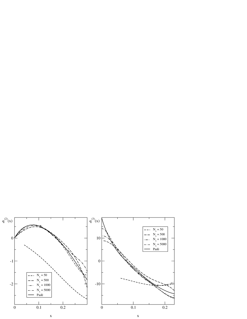
Figure 10: Left panel: second derivative of $q(x)$ at $T=0.6$ and different $N_{x}$. Right panel: third derivative of $q(x)$ at $T=0.6$ and different $N_{x}$. In both cases $x_{0}=1$, $y_{\rm max}=48$ and $N_{y}=4096$. The full line is the perturbative result.

We conclude this Section with a short discussion on the entropy which, using the stationarity of the free energy functional (13), can be written as:

$$s=-\frac{\beta^{2}}{4}\bigl{[}1-q(1)\bigr{]}^{2}+\int_{-\infty}^{\infty}dy\ P(1,y)\bigl{[}\log 2\cosh\beta y-y\ \tanh(\beta y)\bigr{]}.$$ (42)

For other equivalent forms see, e.g., Ref. Luca . The entropy as function of temperature is shown in the left panel of Figure 11. The entropy must vanish quadratically with the temperature as $T\to 0$ SDJPC84 . From our numerical data we find

$$\lim_{T\to 0}\frac{s(T)}{T^{2}}=a\simeq 0.72$$ (43)

to be compared with $0.718\pm 0.004$ of the analytic expansions.

In the limit $T\to 0$ the quantity $1-q(1)$ must also vanish as $T^{2}$ SDJPC84 . The behaviour of $q(1)$ as function of $T$ is shown in the right panel of Figure 11. Using this data we obtain

$$\lim_{T\to 0}\frac{1-q(1)}{T^{2}}\simeq 1.60$$ (44)

in very good agreement the value $1.60\pm 0.01$ obtained with the expansions of previous sections.

Figure 11: Left panel: entropy $s$ as function of temperature $T$. Right panel: $q(1)$ as function of temperature $T$.

VI Conclusions

In this paper we have studied the properties of the $\infty$-replica symmetry breaking solution of the Sherrington - Kirkpatrick model without external fields. Using high order expansions in $\tau=T_{c}-T$ we are able to compute the order parameter $q(x)$ and other relevant quantities for a large range of temperatures with high precision. In particular we found that $q(x)$ is not an odd function of $x$, confirming the prediction of Ref. Temes . Direct consequence of this is that the overlap probability distribution function $P(q)$ has discontinuous derivatives at $q=0$. Another consequence of our findings is that the Parisi-Toulouse scaling becomes exact asymptotically for $T\to 0$ and $\beta x\to 0$, while for $T\to 0$ is a fairly good approximation. This is also consistent with the $T=0$ limit of the breaking point which we found to be $x_{max}(0)=.548\pm.005$.

Having reached very high orders we can reasonably speculate on the analytical properties of the function $q(x)$. In particular we believe that

• All the expansions in power of $\tau$ are asymptotic expansions.

• At any temperature, the function $q(x)$ is infinitely differentiable but not analytical for any $x$, in particular the Taylor expansion of the function $q(x)$ around any $0<x<x_{max}$ does not converge but is asymptotic.

This singular behaviour is not connected neither with the replica limit nor with the Parisi Ansatz, actually it originates from the singularities in the complex plain of the initial condition of the Parisi equation: $f(1,y)=\ln 2\cosh\beta y$. This is clearly seen for the replica-symmetric solution

$$q=\int^{+\infty}_{-\infty}\frac{dz}{\sqrt{2\pi}}e^{\frac{z^{2}}{2}}\tanh^{2}(\beta\sqrt{q}z)$$

In this case it is easy to prove that the expansion of $(1-T^{2})$ in powers of $p=\beta^{2}q$ is asymptotic because it corresponds to substitute $\tanh^{2}z$ in the integrand with its Taylor expansion which is not convergent on the whole real axes. Then one can prove that the expansion of $q$ in powers of $\tau=1-T$ is asymptotic recalling that standard manipulation (e.g. multiplication, division, inversion…) on an asymptotic expansion in power series do not change its character. A detailed treatment of the RSB solution is much more complex, but the origin of the asymptotic character is likely to be the same. Indeed an expansion in small $\tau$ (and therefore in small $q$) corresponds to an expansion in small $y$ of all the quantities like $f(x,y)$ and $m(x,y)$; the appearance of integrals of the form $\int Pfdy$where $P(x,y)\sim\exp(y^{2}/x)$ generates asymptotic expansions since the Taylor expansions of $f(x,y)$ and $m(x,y)$ in powers of $y$ do not converge on the whole real axes. These arguments can be very useful in practice to guess the position of the singularities of the Borel transform if one want to sum the expansions through a conformal mapping Pbook . For instance in the expression of the free energy appear integrals of the following form:

$$\int^{+\infty}_{-\infty}\frac{dz}{\sqrt{2\pi\tau}}e^{-\frac{z^{2}}{2\tau}}\ln\cosh(z)$$ (45)

The singularities of the Borel transform of the previous integral are located on a cut running from $-\infty$ to $-\pi^{2}/8$ and a possible guess is that this be also the singularity structure of the Borel transform of the free energy. This guess is supported by the analysis of the series expansions.

The analytical results have been compared with numerical solutions of the $\infty$-replica symmetry breaking equations. We have developed a new numerical approach based on a pseudo-spectral code which leads to a strong enhancement of the quality of the numerical results. We have also shown how, for example, to determine the value of $x_{\rm max}$ numerically. In all cases the agreement between the numerical and the analytical results is rather good.

We conclude by stressing that our results go beyond the interest on the Sherrington - Kirkpatrick model, since the method we used here are far more general and can be employed to a wider class of models with generalized $\infty$-replica symmetry breaking equations such as those introduced in Ref. Luca . In particular in this reference the numerical method was applied to the 3-SAT model, and the extension to other relevant models is under development.

References

- (1) M. Mezard, G. Parisi, M.Virasoro, Spin Glass Theory and Beyond, World Scientific, Singapore (1987).
- (2) K.H. Fischer and J.A. Hertz, Spin-Glasses (Cambridge University Press, 1991)
- (3) A. Crisanti, L. Leuzzi and G. Parisi, J. Phys. A: Math. Gen. 35, 481 (2002).
- (4) E. Gardner, Nucl. Phys. B257, 747 (1985);
- (5) T.R. Kirkpatrick and D. Thirumalai, Phys. Rev. B 36, 5388 (1987).
- (6) M. Sellitto, M. Nicodemi and J.J. Arenzon J. Phys. I France 7, 945 (1997).
- (7) G. Parisi, Phys. Rev. Lett. 43, 1754 (1979); J. Phys. A 13, L115 (1980).
- (8) I. Kondor, J. Phys. A 16, L127 (1983).
- (9) H.-J. Sommers, J. Physique Lett. 46, L-779 (1985).
- (10) J. Vannimenus, G. Toulouse and G. Parisi J. Physique 42, 565 (1981).
- (11) H. J. Sommers, W. Dupont, J. Phys. C 17 (1984) 5785-5793.
- (12) K. Nemoto, J. Phys. C 20, 1325 (1987).
- (13) P. Biscari, J. Phys. A 23, 3861 (1990)
- (14) T. Temesvari, J. Phys. A 22, L1025 (1989).
- (15) C. De Dominicis and A.P. Young, J. Phys. A 16, 2063 (1983);
- (16) G. Parisi, Phys. Rev. Lett. 50, 1946 (1983).
- (17) G. Parisi, J. Phys. A 13, L115 (1980).
- (18) G. Parisi and Toulouse, J. Physisque Lett. 41, L-361 (1980).
- (19) C.M. Bender and S.A. Orszag, Advanced Mathematical Methods for Scientists and Engineers, McGraw-Hill (1978).
- (20) We note that it is possible to impose a null derivative at directly into the Padè approximants. This however does not produce a sensible improvement of the precisions at a given order, making at the same time more difficult to have a control on the convergence.
- (21) S. A. Orszag, Studies in applied mathematics (Cambridge University, Cambridge, 1971), Vol. 4, p 293.
- (22) G. S. Patterson and S. A. Orszag, Phys. Fluids 14, 2538 (1971)
- (23) See, e.g., J.H. Ferziger and M. Perić, Computational Methods for Fluid Dynamics, Springer-Verlag (1996).
- (24) G. Parisi, Statistical Field Theory, Addison Wesley (1988)