Colloids, polymers, and needles: Demixing phase behavior

Abstract

We consider a ternary mixture of hard colloidal spheres, ideal polymer spheres, and rigid vanishingly thin needles, which model stretched polymers or colloidal rods. For this model we develop a geometry-based density functional theory, apply it to bulk fluid phases, and predict demixing phase behavior. In the case of no polymer-needle interactions, two-phase coexistence between colloid-rich and -poor phases is found. For hard needle-polymer interactions we predict rich phase diagrams, exhibiting three-phase coexistence, and reentrant demixing behavior.

I Introduction

The richness of phase behavior of systems with purely repulsive interactions depends crucially on the number of components. For a one-component system like colloidal hard spheres, there occurs a freezing transition from a single fluid phase to a dense crystal. Adding a second component, such as non-adsorbing globular polymer coilsasakura54 , or rod-like particlesvliegenthart99 ; kluijtmans00 generates an effective depletion-induced attraction between colloidal spheres, leading to the possibility of demixing. This transition is an analog of the vapor-liquid transition in simple fluids: The phase that is concentrated in one of the components corresponds to a liquid, while the dilute phase corresponds to a vapor, and one frequently refers to such phases as colloidal liquid and colloidal vapor, although the “vapor” is concentrated in the added component.

Generic theoretical models for such systems are those introduced by Asakura and Oosawa (AO) and independently by Vrijasakura54 ; vrij76 , Bolhuis and Frenkel (BF)bolhuis94 , and Widom and Rowlinson (WR)widom70 . The AO model comprises hard colloidal spheres mixed with polymer spheres that are ideal amongst themselves but cannot penetrate the colloids. The BF model adds stiff vanishingly thin needles to a hard sphere system. Because of their vanishing thickness, the needles do not interact with one another. Clearly, both models are similar in spirit, as a non-interacting component is added to hard spheres. In the WR model this is different; two species of spheres interact symmetrically, such that hard core repulsion occurs only between particles of unlike species. Hence a pure system of either component is an ideal gas. All of these model binary mixtures exhibit liquid-vapor phase separation, well-established by computer simulations and theories gast83 ; lekkerkerker92 ; dijkstra99 ; louis99 ; dijkstra00I ; brader01phd . The WR modelwidom70 ; guerrero76 ; rowlinson80 ; rowlinson82 has been studied with a range of approaches, including mean-field theory (MFT)rowlinson82 , Percus-Yevick (PY) integral equation theoryrowlinson80 ; shew96 ; yethiraj00 , scaled-particle theory (SPT) bergmann76 , as well as computer simulationsshew96 ; johnson97 ; borgelt90 . The precise location of the liquid-vapor critical point was located by simulations about 50 percent higher than previously thoughtshew96 ; johnson97 , still a challenge for theories (for a recent integral-equation closure, see Ref. yethiraj00 ).

In the AO and BF cases a reservoir description has proven to be useful. The reservoir density of either polymers or needles rules the strength of effective attraction and hence plays a role similar to (inverse) temperature in simple substances. Although the WR model features an intrinsic symmetry which seems to preclude such a description, an effective model can also be formulatedrowlinson82 . In the present work we consider the phase behavior of a mixture of spheres, polymers and needles, a natural combination of the above binary cases. We note that our ternary model may provide insight into certain real systems, such as paints, which contain colloidal latex and pigment particles, polymer thickeners and dispersants, as well as many other componentssatas91 .

Density functional theory (DFT)evans92 is a powerful approach to equilibrium statistical systems, possibly under influence of an external potential. Building on Rosenfeld’s workRosenfeld89 , a geometry-based approach was recently proposed that also predicts bulk properties, without the need of any input, allowing the AOschmidt00cip , BFschmidt01rsf , and WRschmidt01wr models to be treated. Here we combine these tools to derive a DFT for ternary systems.

In Sec. II we define the model ternary mixtures of spheres, polymers, and needles. In Sec. III the DFT is developed. Application to bulk phases in Sec. IV yields the phase behavior. We finish with concluding remarks in Sec. V.

II The Model

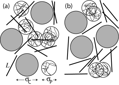
Figure 1: Sketch of the ternary mixture of colloidal hard spheres with diameter $\sigma_{C}$, ideal polymer spheres of diameter $\sigma_{P}$ and vanishingly thin needles of length $L$. Different cases for interactions between polymers and needles are depicted: a) no interactions; b) excluded volume interactions.

We consider a mixture of colloidal hard spheres (species $C$) of radius $R_{C}$, globular polymers (species $P$) of radius $R_{P}$, and vanishingly thin needles (species $N$) of length $L$, with respective number densities $\rho_{C}({\bf r})$, $\rho_{P}({\bf r})$ and $\rho_{N}({\bf r},{\bf\Omega})$, where ${\bf r}$ is the spatial coordinate and ${\bf\Omega}$ is a unit vector pointing along the needle axis (see Fig. 1). The pair interaction between colloids is $V_{CC}=\infty$ if the separation $r$ between sphere centers is less than $2R_{C}$, and zero otherwise. The pair interactions between like particles of both other components vanish for all distances: $V_{PP}=V_{NN}=0$. For polymers this is an assumption strictly valid only at the theta point; for needles it becomes exact in the present limit of large aspect ratio, where overlapping needles contribute a negligible fraction of configurations. The colloidal spheres interact with both other components via excluded volume: The pair interaction between colloids and polymers is $V_{CP}=\infty$ if $r<R_{C}+R_{P}$, and zero otherwise; the interaction between colloids and needles is $V_{CN}=\infty$, if both overlap, and zero otherwise. What remains to be prescribed is the interaction between needles and polymers. We consider two cases: i) ideal interactions such that $V_{PN}=0$ for all distances, and ii) excluded volume interactions such that $V_{PN}=\infty$ if needle and polymer overlap, and zero otherwise. We denote the sphere diameters by $\sigma_{C}=2R_{C}$, $\sigma_{P}=2R_{P}$, the sphere packing fractions by $\eta_{C}=4\pi R_{C}^{3}\rho_{C}/3$, $\eta_{P}=4\pi R_{P}^{3}\rho_{P}/3$, and use a dimensionless needle density $\rho_{N}^{\ast}=\rho_{N}L^{3}.$

III Density functional theory

III.1 Weight functions

We start with a geometrical representation of the particles in terms of weight functions $w_{\mu}^{i}$, where $\mu=3,2,1,0$ corresponds to the particles’ volume, surface, integral mean curvature and Euler characteristic, respectivelyrosenfeld94convex , and $i=C,P,N$ labels the species. We will use $S$ as a unifying symbol for the spherical species $C$ and $P$, and denote the radius as $R$, where $R=R_{C},R_{P}$ for $S=C,P$, respectively. The weight functions are determined to give the hard core Mayer bonds $f_{ij}=\exp(V_{ij})-1$ by a linear combination of terms $w_{\gamma}^{i}({\bf r})*w_{3-\gamma}^{j}({\bf r})$, where the star denotes the convolution, $g({\bf r})*h({\bf r})=\int{\rm d}^{3}x\,g({\bf x})h({\bf r}-{\bf x})$.

For spheres, the usual weight functionsRosenfeld89 ; tarazona00 are

$$w_{3}^{S}({\bf r})= \theta(R-r),\hskip 8.53581ptw_{2}^{S}({\bf r}) =\delta(R-r),$$ (1)

$${\bf w}_{{{\rm v}2}}^{S}({\bf r})= w_{2}^{S}({\bf r})\,{\bf r}/r,\hskip 8.53581pt{\bf\hat{w}}_{{{\rm m}2}}^{S}({\bf r}) =w_{2}^{S}({\bf r})[{\bf r}{\bf r}/r^{2}-{\hat{\mathbf{1}}}/3],$$ (2)

where $r=|{\bf r}|$, $\delta(r)$ is the Dirac distribution, $\theta(r)$ is the step function, and ${\hat{\mathbf{1}}}$ is the identity matrix. Further linearly dependent weights are $w_{1}^{S}({\bf r})=w_{2}^{S}({\bf r})/(4\pi R),{\bf w}_{{{\rm v}1}}^{S}({\bf r})={\bf w}_{{{\rm v}2}}^{S}({\bf r})/(4\pi R),w_{0}^{S}({\bf r})=w_{1}^{S}({\bf r})/R$. Note that these weights have different tensorial rank: $w_{0}^{S}$, $w_{1}^{S}$, $w_{2}^{S}$, $w_{3}^{S}$ are scalars; ${\bf w}_{{{\rm v}1}}^{S}$, ${\bf w}_{{{\rm v}2}}^{S}$ are vectors; ${\bf\hat{w}}_{{{\rm m}2}}^{S}$ is a (traceless) matrix. These functions give the Mayer bond between pairs of spheresRosenfeld89 through $-f_{SS}/2=w_{3}^{S}*w_{0}^{S}+w_{2}^{S}*w_{1}^{S}-{\bf w}_{{{\rm v}2}}^{S}*{\bf w}_{{{\rm v}1}}^{S}$. However, they are not sufficient to recover the sphere-needle Mayer bondrosenfeld94convex . This is achieved through

$$w_{2}^{{\rm\it SN}}({\bf r},{\bf\Omega})=2|{\bf w}_{{{\rm v}2}}^{S}({\bf r})\cdot{\bf\Omega}|,$$ (3)

which contains information about both species: it is non-vanishing on the surface of a sphere with radius $R$, but this surface is “decorated” with an ${\bf\Omega}$-dependence. Furthermore, for needles, we followrosenfeld94convex to obtain

$$w_{1}^{N}({\bf r},{\bf\Omega}) = \frac{1}{4}\int_{-L/2}^{L/2}{\rm d}l\,\delta({\bf r}+{\bf\Omega}\,l),$$ (4)

$$w_{0}^{N}({\bf r},{\bf\Omega}) = \frac{1}{2}\left[\delta({\bf r}+{\bf\Omega}L/2)+\delta({\bf r}-{\bf\Omega}L/2)\right],$$ (5)

and ${\bf r}$ is the needle center of mass. The function $w_{1}^{N}$ describes the linear extent of a needle, whereas $w_{0}^{N}$ is characteristic of its endpoints. For vanishingly thin needles, both surface and volume vanish, and so do the corresponding weights, $w_{2}^{N}=w_{3}^{N}=0$. Technically, the Mayer bond is generated through $-f_{{\rm\it SN}}({\bf r},{\bf\Omega})=w_{3}^{S}({\bf r})*w_{0}^{N}({\bf r},{\bf\Omega})+w_{2}^{{\rm\it SN}}({\bf r},{\bf\Omega})*w_{1}^{N}({\bf r},{\bf\Omega})$, where ${\bf r}$ is the difference vector between sphere and needle position.

III.2 Weighted densities

The weight functions are used to smooth the possibly highly inhomogeneous density profiles by convolutions,

$$n_{\nu}^{C}({\bf r}) = \rho_{C}({\bf r})*w_{\nu}^{C}({\bf r}),$$ (6)

$$n_{\nu}^{P}({\bf r}) = \rho_{P}({\bf r})*w_{\nu}^{P}({\bf r}),$$ (7)

$$n_{2}^{CN}({\bf r},{\bf\Omega}) = \rho_{C}({\bf r})*w_{2}^{CN}({\bf r},{\bf\Omega}),$$ (8)

$$n_{2}^{PN}({\bf r},{\bf\Omega}) = \rho_{P}({\bf r})*w_{2}^{PN}({\bf r},{\bf\Omega}),$$ (9)

$$n_{\tau}^{N}({\bf r},{\bf\Omega}) = \rho_{N}({\bf r},{\bf\Omega})*w_{\tau}^{N}({\bf r},{\bf\Omega}),$$ (10)

where $\nu=0,1,2,3,v1,v2,m2$, and $\tau=0,1$; $\rho_{C}({\bf r})$, $\rho_{P}({\bf r})$ and $\rho_{N}({\bf r},{\bf\Omega})$ are the one-body density distributions of spheres, polymers and needles, respectively. Note that $n_{\nu}^{C},n_{\nu}^{P},n_{\nu}^{N}$ are “pure” weighted densities, involving only variables of either speciesRosenfeld89 ; rosenfeld94convex . In contrast, $n_{2}^{CN}$ and $n_{2}^{PN}$ are a convolution of the sphere densities with orientation-dependent weight function, combining characteristics of both speciesschmidt01rsf .

III.3 Free energy density

The Helmholtz excess free energy is obtained by integrating over a free energy density,

$$F_{\rm exc}[\rho_{C},\rho_{P},\rho_{N}]=k_{\rm B}T\int{\rm d}^{3}x\int\frac{{\rm d}^{2}\Omega}{4\pi}\,\Phi\left(\{n_{\gamma}^{i}\}\right),$$ (11)

where $k_{\rm B}$ is Boltzmann’s constant, $T$ is temperature, and the (local) reduced excess free energy density $\Phi$ is a simple function (not a functional) of the weighted densities $n_{\gamma}^{i}$. This leads to a dependence of $\Phi$ on orientation and position. The variable ${\bf x}$ runs over spaceRosenfeld89 ; rosenfeld94convex , and ${\bf\Omega}$ over the unit sphereschmidt01rsf .

The functional form of $\Phi$ is obtained by consideration of the exact zero-dimensional excess free energy. We obtain

$$\Phi=\Phi_{CC}+\Phi_{CP}+\Phi_{CN}+\lambda\Phi_{PN},$$ (12)

where in the case of ideal polymer-needle interaction $\lambda=0$, and for hard polymer-needle interaction $\lambda=1$. In the following, the arguments of the weighted densities are suppressed in the notation; see Eqs. (6)-(10) for the explicit dependence on ${\bf r}$ and ${\bf\Omega}$. The hard sphere contribution, being equal to the pure HS case Rosenfeld89 ; tarazona00 , is

$$\Phi_{CC} = -n_{0}^{C}\ln(1-n_{3}^{C})+\left(n_{1}^{C}\,n_{2}^{C}-{\bf n}_{{\rm v}1}^{C}\cdot{\bf n}_{{\rm v}2}^{C}\right)/({1-n_{3}^{C}})$$ (13)

$$+\left[{{\left(n_{2}^{C}\right)^{3}}/3}-n_{2}^{C}\,{\left({\bf n}_{{\rm v}2}^{C}\right)^{2}}+3\left({\bf n}_{{\rm v}2}^{C}\cdot{{\hat{\mathbf{n}}}_{{\rm m}2}}^{C}\cdot{\bf n}_{{\rm v}2}^{C}\right.\right.$$

$$\left.\left.\phantom{{\left(n_{2}^{C}\right)^{3}}/3}\left.-\,3\det{{\hat{\mathbf{n}}}_{{\rm m}2}}^{C}\right)/2\right]\right/[8\pi(1-n_{3}^{C})^{2}].$$

The contribution due to interactions between colloids and polymers is the same as in the pure AO caseschmidt00cip and is given by

$$\Phi_{CP}=\sum_{\nu}\frac{\partial\Phi_{CC}}{\partial n_{\nu}^{C}}n_{\nu}^{P}.$$ (14)

The contribution due to interactions between colloids and needlesschmidt01rsf is

$$\Phi_{CN}=-n_{0}^{N}\ln(1-n_{3}^{C})+\frac{n_{1}^{N}n_{2}^{CN}}{1-n_{3}^{C}}.$$ (15)

Note that the simultaneous presence of $\Phi_{CP}$ and $\Phi_{CN}$ in $\Phi$ does not generate artificial interactions between $P$ and $N$. For vanishing $PN$ pair potential one can derive these terms from consideration of multi-cavity distributions like in the binary $CP$schmidt00cip ; brader01phd and $CN$ casesschmidt01rsf . In order to model the WR type interaction between polymers and needles in the presence of the colloidal spheres we use

$$\Phi_{PN}=\frac{n_{0}^{N}n_{3}^{P}+n_{1}^{N}n_{2}^{PN}}{1-n_{3}^{C}}.$$ (16)

This can be derived as follows. The starting point is a functional for binary hard spheres with added needles. Linearization in one of the sphere densities (which becomes the polymer species) is performed in the same way as linearization of binary hard spheres leads to the $CP$ functionalbrader01phd . In the absence of colloids, we obtain $\Phi=\Phi_{CN}=n_{0}^{N}n_{3}^{P}+n_{1}^{N}n_{2}^{PN}$. Then the density functional then can be rewritten as $F_{\rm exc}=-\int d^{3}r\int d^{3}r^{\prime}\int d^{2}\Omega\rho_{P}({\bf r})f_{PN}({\bf r};{\bf r}^{\prime},{\bf\Omega})\rho_{N}({\bf r},{\bf\Omega})/(4\pi)$. This is precisely (a generalization to needles of) the mean-field DFT for the WR modelrowlinson82 . Although this does not feature the exact 0d limit, as the geometry-based DFTschmidt01wr for WR spheres does, we expect differences to be small.

IV Results

IV.1 Bulk fluid phases

For homogeneous density profiles, $\rho_{i}=\rm const$, the integrations in Eqs. (6)-(10) can be carried out explicitly. The hard sphere contribution is equal to the Percus-Yevick compressibility (and scaled-particle) result, which is

$$\Phi_{CC}=\frac{3\eta_{C}[3\eta_{C}(2-\eta_{C})-2(1-\eta_{C})^{2}\ln(1-\eta_{C})]}{8\pi R_{C}^{3}(1-\eta_{C})^{2}}.$$ (17)

The colloid-polymer contribution is equal to that predicted by free volume theorylekkerkerker92 , and rederived by DFTschmidt00cip as

$$\Phi_{CP} = \frac{\eta_{P}/(8\pi R_{P}^{3})}{(1-\eta_{C})^{3}}\left\{3q\eta_{C}\left[6(1-\eta_{C})^{2}+3q(2-\eta_{C}-\eta_{C}^{2})\right.\right.$$ (18)

$$\left.\left.+2q^{2}(1+\eta_{C}+\eta_{C}^{2})\right]-6(1-\eta_{C})^{3}\ln(1-\eta_{C})\right\},$$

where $q=\sigma_{P}/\sigma_{C}$. The colloid-needle contribution equals the perturbative (around a pure hard sphere fluid) treatment of Ref.bolhuis94 , which can be shown to equal the result from application of scaled-particle theorybarker76 , and DFTschmidt01rsf , and is given by

$$\Phi_{CN}=\rho_{N}\left[-\ln(1-\eta_{C})+\ \frac{3L}{4R_{C}}\,\frac{\eta_{C}}{1-\eta_{C}}\right].$$ (19)

The WR type polymer-needle contribution is

$$\Phi_{PN}=\left(1+\frac{3L}{4R_{P}}\right)\frac{\rho_{N}\eta_{P}}{1-\eta_{C}}.$$ (20)

For completeness, the ideal free energy contribution is

$$\Phi_{\rm id}=\sum_{i=C,P,N}\rho_{i}[\ln(\rho_{i}\Lambda_{i}^{3})-1],$$ (21)

where the $\Lambda_{i}$ are (irrelevant) thermal wavelengths of species $i$. This puts us into a position to obtain the reduced total free energy per volume $\Phi_{\rm tot}=\Phi_{\rm id}+\Phi$ of any given fluid state characterized by the bulk densities and relative sizes of the three components.

IV.2 Phase diagram

The general conditions for phase coexistence are equality of the total pressures $p_{\rm tot}$, and of the chemical potentials $\mu_{i}$ in the coexisting phases. Equality of temperature is trivial in hard-body systems. For phase equilibrium between phases I and II,

$$p_{\rm tot}^{\rm I} = p_{\rm tot}^{\rm II}$$ (22)

$$\mu_{i}^{\rm I} = \mu_{i}^{\rm II},\quad i=C,P,N.$$ (23)

These are four equations for six unknowns (two statepoints each characterized by three densities). Hence two-phase coexistence regions depend parametrically on two free parameters. For three-phase equilibrium between phases I, II, and III

$$p_{\rm tot}^{\rm I} = p_{\rm tot}^{\rm II}=p_{\rm tot}^{\rm III}$$ (24)

$$\mu_{i}^{\rm I} = \mu_{i}^{\rm II}=\mu_{i}^{\rm III},\quad i=C,P,N.$$ (25)

Eight equations for nine variables leave one free parameter.

In our case $p_{\rm tot}/k_{B}T=-\Phi_{\rm tot}+\sum_{i=C,P,N}\rho_{i}\partial\Phi_{\rm tot}/\partial\rho_{i}$, and $\mu_{i}=k_{B}T\partial\Phi_{\rm tot}/\partial\rho_{i}$ yield analytical expressions. We solve the resulting sets of equations numerically, which is straightforward.

IV.2.1 Ideal polymer-needle interaction

Let us first explain our representation of the ternary phase diagrams. We take the system densities $\eta_{C},\eta_{P},\rho_{N}^{\ast}$ as basic variables. For given particle sizes, these span a three-dimensional (3d) phase space. Each point in this space corresponds to a possible bulk state, at some pressure $p_{\rm tot}$. Two-phase coexistence is indicated by a pair of points that are joined by a straight tie line. Accordingly, three phase coexistence is a triplet of points, defining a triangle. In order to graphically represent the phase diagram, we show surfaces defined by one thermodynamic parameter being constant. Such surfaces are conveniently taken such that coexistence lines (and triangles) lie completely within the surface. Clearly, this can be accomodated by imposing a constant value of $p_{\rm tot}$ or any of $\mu_{C},\mu_{P}$, and $\mu_{N}$. Here we choose $\mu_{P}=\rm const$, and hence imagine controlling the system directly with $\eta_{C}$ and $\rho_{N}^{\ast}$, but indirectly via coupling to a polymer reservoir of packing fraction $\eta_{P}^{r}=(4\pi/3)(R_{P}/\Lambda_{P})^{3}\exp(\mu_{P}/k_{B}T)$. A constant-$\eta_{P}^{r}$-surface is non-trivially embedded in the 3d phase diagram. To depict it graphically, we show projections onto the three sides of the coordinate system, namely the $\eta_{C}-\rho_{N}^{\ast}$, $\eta_{C}-\eta_{P}$, and $\eta_{P}-\rho_{N}^{\ast}$ planes, as well as a perspective 3d view. Furthermore, we indicate the accessible regions that are compatible with the constraint of fixed $\eta_{P}^{r}$. Their boundaries are implicitly defined through $\eta_{P}^{r}(\eta_{C}=0,\eta_{P},\rho_{N}^{\ast})=\rm const$ and $\eta_{P}^{r}(\eta_{C},\eta_{P},\rho_{N}^{\ast}=0)=\rm const$. Note that tielines are allowed to cross inaccessible regions.

For simplicity, and to establish a reference case, we initially ignore polymer-needle interactions and consider equal particle sizes, $\sigma_{C}=\sigma_{P}=L$. In the absence of polymer ($\eta_{P}^{r}=0$), colloids and needles demix, as shown in Fig. 2a. Increasing the packing fraction of polymers in the reservoir causes the demixed region to grow and to shift to smaller $\eta_{C}$ and $\rho_{N}^{\ast}$ (see Fig. 2b for $\eta_{P}=0.5$). This behavior can be understood if addition of a second depleting species simply enhances the depletion-induced attraction between colloids. Increasing $\eta_{P}^{r}$ further causes the critical point to hit the $\rho_{N}^{\ast}=0$ axis. This is precisely the demixing critical point of the binary $CP$ (AO) model, which is located at $\eta_{P}^{r}=0.63831$ (see Fig. 2c). Computer simulations are currently being carried out to test the accuracy of this valuedijkstra01private . For still larger $\eta_{P}^{r}$, the mixed states become disconnected, hence there is no path between colloid-rich and colloid-poor phases that does not pass through a first-order phase transition (see Fig. 2d for $\eta_{P}^{r}=0.8$).

IV.2.2 Hard polymer-needle interaction

Turning on the excluded volume interaction between polymers and needles allows the possibility of demixing between these components. In the absence of colloids, the $PN$ mixture is of WR type: Interactions between particles of like species vanish, while unlike particles interact with a hard core repulsion. Our case is a generalization to non-spherical particle shapes. In the mean-field treatment this does not affect the phase diagram, as only the net excluded volume enters into the theory. This robustness is also present in our approach.

We first consider equal particle sizes, $\sigma_{C}=\sigma_{P}=L$. It turns out that interesting behavior is observed only for small $\rho_{N}^{\ast}<0.2$. The colloid-needle demixing curve lies well above this region, and is only weakly affected by $\eta_{P}^{r}>0$. In the absence of needles ($\rho_{N}^{\ast}=0$) and for large enough polymer density, colloids and polymers demix, indicated by a miscibility gap along the $\rho_{N}^{\ast}=0$ axis (see Fig. 3a for $\eta_{P}^{r}=0.8$). Increasing needle density $\rho_{N}^{\ast}>0$ causes the gap to shrink and eventually to disappear in a critical point. Quite surprisingly, and in contrast to the former case of absent $PN$ interactions, the addition of needles favors mixing. This behavior may reflect a competition between the depleting effects of interacting polymers and needles. By analogy with the $CP$ subsystem it is clear that at sufficiently high polymer density, a $PN$ miscibility gap will open for $\eta_{C}=0$. However, this happens not by growing a small bump as in the $CP$ case. Instead the $CP$ demixing curve bends over to smaller $\eta_{C}$ and touches (with its critical point) the $\eta_{C}=0$ axis (see Fig. 3b for $\eta_{P}^{r}=1.08731$). For larger $\eta_{P}^{r}$, the critical point disappears (see Fig. 3c for $\eta_{P}^{r}=1.2$).

In order to bring $CP$ and $CN$ demixing closer together, we consider a reduced polymer size $\sigma_{P}=\sigma_{C}/2$, generating a weaker depletion attraction between colloids (at the same number density of polymers), and longer needles, $L=2\sigma_{C}$ generating stronger depletion between colloids, and hence lower $\rho_{N}^{\ast}$ at the critical point in the binary $CN$ case. Figure 4 shows the binodals in the (three) binary subsystems. For the ternary mixture, we follow a path of increasing $\eta_{P}^{r}$, starting with $\eta_{P}^{r}=0$, for which the phase diagram is displayed in Fig. 5a. There is no polymer present in the system, and phase separation into colloid-rich and needle-rich phases occurs at high enough densities of these components. Both $\eta_{P}-\rho_{N}^{\ast}$ and $\eta_{C}-\eta_{P}$ planes are inaccessible as $\eta_{P}=0$. Increasing polymer density ($\eta_{P}^{r}=0.4$ in Fig.5b) shifts the $CN$ critical point to lower $\eta_{C}$, distorting the formerly rounded shape of the binodal. For $\eta_{C}=0$, polymers and needles demix, as $\eta_{P}^{r}$ is above the critical value for the Widom-Rowlinson type demixing of these species. The presence of colloids ($\eta_{C}>0$) disturbs the $PN$-transition; the miscibility gap narrows, eventually disappearing in a critical point, with subsequent miscibility. At $\eta_{P}^{r}=0.408107$ (Fig. 5c) the $CN$ and $PN$ critical points merge into a single one, and a needle-rich phase ($N$) becomes isolated. This coexists with a phase that consists (primarily) of colloids and polymers at varying composition. For growing $\eta_{P}^{r}$, the “double” critical point broadens into a line and results in a thin neck joining both transitions.

With increasing $\eta_{P}^{r}$ the coexistence region broadens further (see Fig. 5d for $\eta_{P}^{r}=0.5$). Colloids and polymers also demix. For $\rho_{N}^{\ast}=0$, the system is above the critical point for the pure AO model, and hence coexistence between colloid-rich and polymer-rich phases occurs. Again, the presence of the third component, in this case $N$, causes the density gap to shrink and eventually disappear with a critical point. As all binary subsystems are by now demixed, it is evident that the system will ultimately display coexistence between three phases, each one enriched by one of the components, and represented by a triangle in system representation. Each corner of the triangle corresponds to one of the three coexisting phases. The Gibbs phase rule dictates that one degree of freedom remains, which is $p_{\rm tot}$ or, equivalently, $\eta_{P}^{r}$ (note that for hard-body systems, temperature is trivially related to pressure). It is striking, however, how this triangle develops. One might expect this to occur by the joining of existing binary coexistence regions. This is not the case. The ternary region instead grows solely out of the $N$-rich–poor coexistence, whereby $CP$-coexistence is only a spectator, separated by mixed states. The initial three-phase triangle is extremely elongated (being a line as a boundary case). One corner corresponds to a needle-rich phase; both others differ only slightly in densities, one phase favoring colloids, the other polymers. Moving away from this $CP$-edge of the triangle (by reducing $\rho_{N}^{\ast}$) leads to binary coexistence between $C$ and $P$. This phase separation is reminiscent of the behavior of the pure AO model. However this reentrant coexistence is triggered by the presence of the needles, and it is separated (by mixed states) from the pure AO transition (and its region of stability in the presence of needles). In Fig. 5e we show results for $\eta_{P}^{r}=0.52626$, where the critical points of both $CP$ transitions have already merged, and again a neck is reminiscent of the formerly distinct transitions. For still larger $\eta_{P}^{r}$, the three-phase triangle grows further (see Fig. 5f for $\eta_{P}^{r}=0.54$). Ultimately, at sufficient concentration the colloids must freeze, but we disregard the solid phase in the present work. We finally note that the whole scenario is covered over a relatively small density interval $\eta_{P}^{r}=0.4-0.54$, and that the packing fractions of colloids and polymers are only moderate. However, needle densities can be quite high.

V Discussion

In conclusion, we have considered a simple hard-body model for a mixture of spherical colloidal particles, globular polymer coils and needle-shaped objects, which may represent either colloidal needles, stretched polymers or polyelectrolytes. We have extended a recent DFT approach to this model and applied it to bulk fluid phases. The resulting phase behavior is very rich, ensuing from competition of demixing in the binary subsystems.

The present work has interesting implications for the techniques of integrating out degrees of freedom (see e.g. brader00 ; brader01inhom ). Note that by integrating out, e.g., the needles, effective interactions between pairs of colloids, pairs of polymers, as well as colloids and polymers arise. Hence one arives at a binary mixture with (soft) depletion interactions. To what extent the ultimate mapping onto a one-component (colloid) system, by further integrating out the polymers, can be achieved is an interesting question. As a further outlook, the inclusion of freezing of colloids, disregarded in the present work, would further enrich the phase behavior. Computer simulations are desirable to test the theoretical phase diagrams. Furthermore it is interesting to elucidate the structural correlations present in the various fluid phases. Inhomogeneous situations, such as induced by walls or present at interfaces between demixed states, constitute further exciting directions of research.

We acknowledge useful discussions with Stuart G. Croll.

*Permanent address: Institut für Theoretische Physik II, Heinrich-Heine-Universität Düsseldorf, Universitätsstraße 1, D-40225 Düsseldorf, Germany.

Figure 2: Demixing phase diagram of a ternary colloid-polymer-needle mixture with ideal polymer-needle interactions for $\sigma_{C}=\sigma_{P}=L$, and $\eta_{P}^{r}=$0 (a), 0.5 (b), 0.63831 (c), 0.8 (d). Shown are binodals (lines), tielines between coexisting phases (thin lines), and critical points (dots).

Figure 3: Demixing phase diagram of a ternary colloid-polymer-needle mixture with hard polymer-needle interactions for $\sigma_{C}=\sigma_{P}=L$, and $\eta_{P}^{r}=$0.8 (a), 1.08731 (b), 1.2 (c).

Figure 4: Demixing phase diagrams in the binary subsystems with hard polymer-needle interactions for $\sigma_{C}=2\sigma_{P}=L/2$.

Figure 5: Same as Fig. 3, but for $\sigma_{C}=2\sigma_{P}=L/2$, and $\eta_{P}^{r}=$0 (a), 0.4 (b), 0.408107 (c), 0.5 (d), 0.52626 (e), 0.54 (f).

References

- (1) S. Asakura and F. Oosawa, J. Chem. Phys. 22, 1255 (1954).
- (2) G. A. Vliegenthart and H. N. W. Lekkerkerker, J. Chem. Phys. 111, 4153 (1999).
- (3) S. G. J. M. Kluijtmans, G. H. Koenderink, and A. P. Philipse, Phys. Rev. E 61, 626 (2000).
- (4) A. Vrij, Pure and Appl. Chem. 48, 471 (1976).
- (5) P. Bolhuis and D. Frenkel, J. Chem. Phys. 101, 9869 (1994).
- (6) B. Widom and J. S. Rowlinson, J. Chem. Phys. 52, 1670 (1970).
- (7) A. P. Gast, C. K. Hall, and W. B. Russell, J. Coll. Int. Sci. 96, 251 (1983).
- (8) H. N. W. Lekkerkerker, W. C. K. Poon, P. N. Pusey, A. Stroobants, and P. B. Warren, Europhys. Lett. 20, 559 (1992).
- (9) M. Dijkstra, J. M. Brader, and R. Evans, J. Phys. Condens. Matter 11, 10079 (1999).
- (10) A. A. Louis, R. Finken, and J. Hansen, Europhys. Lett. 46, 741 (1999).
- (11) M. Dijkstra, R. van Roij, and R. Evans, J. Chem. Phys. 113, 4799 (2000).
- (12) J. M. Brader, Ph.D. thesis, University of Bristol, 2001.
- (13) M. I. Guerrero, J. S. Rowlinson, and G. Morrison, J. Chem. Soc. Faraday Trans. II 72, 1970 (1976).
- (14) J. S. Rowlinson, Adv. Chem. Phys. 41, 1 (1980).
- (15) J. S. Rowlinson and B. Widom, Molecular theory of capillarity (Clarendon Press, Oxford, 1982).
- (16) C. Y. Shew and A. Yethiraj, J. Chem. Phys. 104, 7665 (1996).
- (17) A. Yethiraj and G. Stell, J. Stat. Phys. 100, 39 (2000).
- (18) E. Bergmann, Mol. Phys. 32, 237 (1976).
- (19) G. Johnson, H. Gould, J. Machta, and L. K. Chayes, Phys. Rev. Lett. 79, 2612 (1997).
- (20) P. Borgelt, C. Hoheisel, and G. Stell, J. Chem. Phys. 92, 6161 (1990).
- (21) Coatings Technology Handbook, edited by D. Satas (Marcel Dekker, New York, 1991).
- (22) R. Evans, in Fundamentals of Inhomogeneous Fluids, edited by D. Henderson (Dekker, New York, 1992), p. 85.
- (23) Y. Rosenfeld, Phys. Rev. Lett. 63, 980 (1989).
- (24) M. Schmidt, H. Löwen, J. M. Brader, and R. Evans, Phys. Rev. Lett. 85, 1934 (2000).
- (25) M. Schmidt, Phys. Rev. E 63, 050201(R) (2001).
- (26) M. Schmidt, Phys. Rev. E 63, 010101(R) (2001).
- (27) Y. Rosenfeld, Phys. Rev. E 50, R3318 (1994).
- (28) P. Tarazona, Phys. Rev. Lett. 84, 694 (2000).
- (29) J. A. Barker and D. Henderson, Rev. Mod. Phys. 48, 587 (1976).
- (30) M. Dijkstra (unpublished).
- (31) J. M. Brader and R. Evans, Europhys. Lett. 49, 678 (2000).
- (32) J. M. Brader, M. Dijkstra, and R. Evans, Phys. Rev. E 63, 1405 (2001).