Supersymmetric approach to the infinite U Hubbard Model

Abstract

We present a preliminary discussion on the use of supersymmetric representation of the Hubbard operator which unifies the slave boson and slave fermion representations into a single $U(1)\times SU(1|1)$ gauge theory to treat the physics of the infinite U Hubbard model. By looking for solutions to the Hamiltonian in which the spins can exist as both condensed ordered moments and as mobile charged carriers, we examine the possibility of a Nagaoka ferromagnetic phase at finite doping with a quantum critical point into the paramagnetic phase.

The infinite $U$ Hubbard model[1] is a prototype model for strongly correlated electron systems. Interest in this venerable model has grown in recent times because of its link with one of the basic models of high temperature superconductivity, the $t-J$ model.[2] The infinite $U$ Hubbard model corresponds to the $t-J$ model without antiferromagnetic interactions ($J\rightarrow 0$). Despite the absence of antiferromagnetic interactions, evidence from finite temperature Lanzcos studies[3] suggests that many of high temperature properties associated with the cuprate metals are already present in the infinite $U$ Hubbard model.

The $U=\infty$ Hubbard hamiltonian is written

$$H_{K}=-\frac{t}{N}\sum_{(i,j)}[X_{\sigma 0}(i){\rm X}_{0\sigma}(j)+{\rm H.c}]-\mu\sum_{j}{N}_{j}\ .$$ (1)

Here, the Hubbard operators $X_{ab}=|a><b|$ where $|a\rangle\in\{|0\rangle,\{|\sigma\rangle\}\}$ describes a set of atomic states involving a charged “hole” $|0\rangle$ or a neutral spin state $|\sigma\rangle$ with spin component $\sigma\in\{1\dots N\}$ which for generality can have one of $N$ possible values. $a,b\in{|0\rangle,|\sigma\rangle}$

Thouless and Nagaoka [4, 5] first established that the ground state of the half filled $U=\infty$ Hubbard model doped with one hole is a fully saturated ferromagnet. A wide body of theoretical work[6, 7, 8, 9, 10] suggests that ferromagnetism remains stable to a finite hole doping, but there is no consensus about how it evolves and ultimately decays into the paramagnetic state. In particular:

• Does a fully polarized state with $M=1-x$ survive to a finite doping, or is $M<(1-x)$ for all doping?

• Is the transition to the paramagnet second order with a quantum critical point, or is it first order?

For the 2D square lattice variational studies give a critical doping $\delta_{c}\simeq 0.22\relbar 0.49$ [8]. High temperature expansions [9] find that $\delta_{c}\simeq 3/11$ with no region of fully saturated magnetization, yet recent variational Monte Carlo studies [10] suggest that a partially polarized ferromagnet survives between $\delta_{1}\simeq 0.16$ and a quantum critical point (QCP) into the paramagnet at $\delta_{2}\simeq 0.40$.

There are two well-known approaches to incorporating the $U=\infty$ constraint of the Hubbard operators: the slave boson, and the slave fermion approach.[11] A mean-field slave fermion approach [11] leads to the conclusion that he infinite $U$ Hubbard model has a stable ferromagnetic ground state for all doping, while using a slave bosons representation, the system is paramagnetic for all dopings.

In this paper we use a supersymmetric representation of Hubbard operators, given by

$$X_{\sigma\sigma^{\prime}} = b^{\dagger}_{\sigma}b_{\sigma^{\prime}}+f^{\dagger}_{\sigma}f_{\sigma^{\prime}}$$ (2)

$$X_{\sigma 0} = b^{\dagger}_{\sigma}\chi+f^{\dagger}_{\sigma}\phi,\qquad X_{0\sigma}=\chi^{\dagger}b_{\sigma}+\phi^{\dagger}f_{\sigma}$$ (3)

$$X_{00} = \chi^{\dagger}\chi+\phi^{\dagger}\phi\ .$$ (4)

This unifies the slave bosons and slave fermion approach into a single $U(1)\times SU(1|1)$ gauge theory [12]. Two constraints make the representation irreducible

$$Q = n_{{b}}+n_{{\phi}}+n_{{f}}+n_{{\chi}}$$

$$Y = n_{{\phi}}+n_{{f}}-(n_{{b}}+n_{{\chi}})+\frac{1}{Q}[\theta,\theta^{\dagger}]\ ,$$ (5)

where $\theta=\sum_{\sigma}{b}_{\sigma}^{\dagger}{f}_{\sigma}-{\chi}^{\dagger}{\phi}$. The operators $\theta$ ,$\theta^{\dagger}$, $Q$ and $Y$ commute with the constraints and Hubbard operators, generating a local $SU(1|1)$ supersymmetry. For the $S=1/2$ Hubbard model, we must choose $Q=1$ and $Y=0$. A new feature is the appearance of a “superspin”

$$\tau_{3}=\frac{1}{Q}[\theta^{\dagger},\theta]$$

which takes the values $+1$ and $-1$ in pure slave boson ($+1$) or slave fermion representation ($-1$), lying between these extremes in a partially polarized ferromagnet.

Consider the coherent state $|b,\phi\rangle=\exp[\sum_{j}b\hat{b}^{\dagger}_{j\uparrow}+\phi\hat{\phi}^{\dagger}_{j}]|0\rangle$ in which the “up” Schwinger boson and slave boson are condensed, where $|0\rangle$ is the state with one $\chi$ fermion per site and $b$ and $\phi$ are c-numbers. The action of the Hubbard operator on $|b,\phi\rangle$ is given by

$$X_{\sigma o}({\bf k})|b,\phi\rangle=(\delta_{{\sigma\uparrow}}b\hat{\chi}^{\dagger}_{{\bf k}}+\phi\hat{f}^{\dagger}_{{{\bf k}\sigma}})|b,\phi\rangle,$$ (6)

where $X_{\sigma o}(j)=\frac{1}{\sqrt{N}}\sum_{j}X_{\sigma o}(j)e^{-i{\bf k}\cdot{\bf x}_{j}}$ is the Fourier transform of the Hubbard operator. If we now construct a Gutzwiller wavefunction with Fermi momenta $k_{F\uparrow}$ and $k_{F\downarrow}$ for the up and down electrons, we obtain

$$|\psi\rangle = {\mathcal{P}}_{G}\prod_{k<k_{F\sigma},\sigma}X_{\sigma o}({\bf k})|b,\phi\rangle$$ (7)

$$= {\mathcal{P}}_{G}\prod_{k<k_{F\sigma},\sigma}(b\chi^{\dagger}_{\vec{k}}\delta_{{\sigma\uparrow}}+\phi f^{\dagger}_{\vec{k\sigma}})|b,\phi\rangle$$ (8)

where ${\mathcal{P}}_{G}$ is the projection operator that imposes $(Q,Y)=(1,0)$ on each site.

Here we outline an exploration of this wavefunction using analytic methods. To simplify matters we transform to a gauge called the $\chi$ gauge in which the fermi field associated with the constraint is absorbed into the slave fermion $\chi$. Details of this transformation will be provided in a future publication. The constraints in the $\chi$ gauge for $S=1/2$ become $Q=N_{F}+N_{B}=1$ and $Y=N_{F}-N_{B}+\tau_{3}(\zeta)=0$, where $N_{F}=n_{f}+n_{\varphi}$, $N_{B}=n_{b}+n_{\chi}$, $\tau_{3}(\zeta)=-\tanh(\zeta\beta)$ is the expectation value of the superspin $\hat{\tau}_{3}$ and $\zeta$ is the chemical potential conjugate to $Y$. In other words

$$N_{F} = \frac{1}{2}(1+\tau_{3}(\zeta))$$

$$N_{B} = \frac{1}{2}(1-\tau_{3}(\zeta))\ .$$ (9)

If $\zeta\neq 0$, then in the ground-state $\tau_{3}=-sgn(\zeta)$. corresponding to a fully polarized slave fermion phase or a paramagnetic slave boson phase. However, the case $\lim_{T\rightarrow 0}\zeta=0$ allows a new phase where both slave bosons and slave fermions coexist and $-1<\tau_{3}<1$.

Here we describe a mean field approach in which the constraint field $\chi$ is be approximated in a single sharp mode. We briefly describe the results of this analysis in 2D. Carrying out a particle-hole transformation on the field $\chi\rightarrow-\tilde{\chi}^{\dagger}$, the mean field hamiltonian is

$$H_{MF} = \sum_{k}(f^{\dagger}_{k,\sigma},\chi^{\dagger}_{\bf k})\left[\matrix{t_{\bf k}\phi^{2}+\lambda_{f}&t_{\bf k}\phi b\cr t_{\bf k}&t_{k}b^{2}+\lambda_{\chi})}\right]\left(\matrix{f_{k,\sigma}\cr\chi_{\bf k}}\right)$$ (10)

$$+ (\lambda+\zeta)\varphi^{2}+(\lambda-\zeta-\mu)b^{2}-\zeta(\tau_{3}-1),$$ (11)

where $t_{k}=-2t\cos k_{x}+\cos k_{y}$, $\lambda_{f}=\lambda+\zeta-\mu$, $\lambda_{\chi}=\zeta-\lambda$. Note the hybridization between the electron and spinless hole $\chi$ which develops when $\phi b\neq 0$.

We find that the mean-field Free energy $E-\mu N$ of the paramagnetic ($\zeta>0$) and fully polarized ground-state ($\zeta<0$) become equal at a chemical potential $\mu^{*}=0.77t$, corresponding to two different dopings $(\delta_{1},\delta_{2})=(0.25,0.45)$. Varying $\tau_{3}$ at $\mu=\mu^{*}$, we find that the point where $\zeta=dF/d\tau_{3}=0$ is a local maximum (Fig 1 (b)), corresponding to a phase separation between the paramagnetic and fully polarized phases between $\delta_{1}$ and $\delta_{2}$. (Fig. 1 ) Unlike recent results of Bocca and Sorella, there is no QCP at $x=\delta_{2}$.

Perhaps the most interesting result from this analysis, is the discovery that the transition from the magnet to the paramagnet may occur via a phase where $\zeta=0$, raising the fascinating possibility that the magnetic quantum critical point involves soft supersymmetric gauge fluctuations. In future work, we hope to examine whether the self-energy of the $\chi$ field and the fluctuations in $\zeta$ can stabilize a second-order QCP.

We should particularly like to thank A. M. Tremblay and J. Hopkinson for early discussions related to this work. Discussions with W. Puttika and J. Hopkinson are also gratefully acknowledged. Part of this work was carried out at the Aspen Center for Physics. This work was supported in part by the National Science Foundation under grant DMR 9983156 (PC).

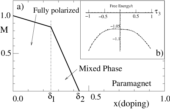
Figure 1: (a)Magnetization as a function of doping in mean field theory. Inset (b) showing variation of free energy with $\tau_{3}$, showing that a partially polarized state is unstable w.r.t. phase separation.

References

- [1] J. Hubbard, Proc. R. Soc. London Ser. A.277, 237 (1964)
- [2] See T. M Rice, in Les Houches LVI, 1991 edited by B. Doucot and J. Zinn-Justin (Elsevier, 1995), p. 19.
- [3] J. Jaklic and P. Prelovsek, Phys. Rev. Lett. 77, 882 (1996).
- [4] D. J. Thouless, Proc. Phys. Soc. London 86,893 (1965).
- [5] Y. Nagaoka, Phys. Rev. 147, 392 (1996); D. J. Thouless, Proc. Phys. Soc. 86, 83 (1965).
- [6] J. Kanamori, Prog. Theor. Phys. 30, 275 (1963).
- [7] W. von der Linden and D. Edwards, J. Phys: Cond. Mat. 3,4917 (1991);X. Y. Zhang et al., Phys. Rev. Lett. 66, 1236 (1991).
- [8] B. S. Shastry et al. Phys. Rev. B 41, 2375 (1990); A. G. Basile et al., Phys. Rev. B 41, 4842 (1990); E. Muller-Hartmann —it et al., Physica B 186-188, 834 (1993).
- [9] W.O. Putikka et al., Phys. Rev. Lett. 69, 2288 (1992).
- [10] F. Becca and S. Sorella, Cond-Mat/0102249.
- [11] D. Boies, F. A. Jackson and A-M. S. Tremblay, Int. Jour. Mod. Phys B 9, 1001 (1995).
- [12] P. Coleman, C. Pépin and A. M. Tsvelik, Phys. Rev. B 62 3852 (2000); P. Coleman, C. Pépin and J . Hopkinson, Phys. Rev. B 63,140411R (2001).