Towards a Macroscopic Modelling of the Complexity in Traffic Flow

Abstract

Based on the assumption of a safe velocity $U_{\rm e}(\rho)$ depending on the vehicle density $\rho$ a macroscopic model for traffic flow is presented that extends the model of the Kühne-Kerner-Konhäuser by an interaction term containing the second derivative of $U_{\rm e}(\rho)$. We explore two qualitatively different forms of $U_{\rm e}$: a conventional, Fermi-type function and, motivated by recent experimental findings, a function that exhibits a plateau at intermediate densities, i.e. in this density regime the exact distance to the car ahead is only of minor importance. To solve the fluid-like equations a Lagrangian particle scheme is developed.
The suggested model shows a much richer dynamical behaviour than the usual fluid-like models. A large variety of encountered effects is known from traffic observations many of which are usually assigned to the elusive state of “synchronized flow”. Furthermore, the model displays alternating regimes of stability and instability at intermediate densities, it can explain data scatter in the fundamental diagram and complicated jam patterns. Within this model, a consistent interpretation of the emergence of very different traffic phenomena is offered: they are determined by the velocity relaxation time, i.e. the time needed to relax towards $U_{\rm e}(\rho)$. This relaxation time is a measure of the average acceleration capability and can be attributed to the composition (e.g. the percentage of trucks) of the traffic flow.

I Introduction

Traffic is a realization of an open one-dimensional many-body system. Recently, Popkov and Schütz popkov99 found that the fundamental diagram determines the phase diagram of such a system, at least for a very simple, yet exactly solvable toy model, the so called asymmetric exclusion process (ASEP). In particular, the most important feature that influences the phase diagram is the number of extrema in the fundamental diagram.

This is exactly the theme of this report. We present an extension of classical, macroscopic (“fluid-like”) traffic flow models. Usually, it is assumed that the fundamental diagram is a one-hump function, however recent empirical results point to more complicated behaviour. It is impossible to assign a single flow function $j(\rho)$ to the measured data-points in a certain density range. Therefore, it can be speculated, that this scatter hides a more complicated behaviour of the fundamental diagram in this regime. We explore two qualitatively different forms of the safe velocity $U_{e}(\rho)$, the velocity to which the flow tends to relax, which leads from the usual one-hump behaviour of the flow density relation to a more complicated function that exhibits, depending on the relaxation parameter, one, two or three humps. Obviously, real drivers may have different $U_{e}(\rho)$–functions, adding another source of dynamical complexity, which will not be discussed in this paper.

II The Model

II.1 Equations

If the behaviour of individual vehicles is not of concern, but the focus is more on aggregated quantities (like density $\rho$, mean velocity $v$ etc.), one often describes the system dynamics by means of macroscopic, fluid-like equations. The form of these Navier-Stokes-like equations can be motivated from anticipative behaviour of the drivers.
Assume there is a safe velocity $U_{e}$ that only depends on the density $\rho$. The driver is expected to adapt the velocity in a way that $v$ relaxes on a time scale $\tau$ to this desired velocity corresponding to the density at $x+\Delta x$,

$$v(x+v\tau,t+\tau)=U_{e}(\rho(x+\Delta x)).$$ (1)

If both sides are Taylor-expanded to first order one finds

$$v(x)+\frac{\partial v}{\partial x}v\tau+\frac{\partial v}{\partial t}\tau+O(\tau^{2})=U_{e}(\rho)+\frac{\partial U_{e}}{\partial\rho}\frac{\partial\rho}{\partial x}\Delta x+O((\Delta x)^{2}).$$ (2)

Inserting $\Delta x=\rho^{-1}$

$$\frac{\partial v}{\partial t}+v\frac{\partial v}{\partial x}=\frac{U_{e}(\rho)-v}{\tau}+\frac{1}{\rho\tau}\frac{\partial U_{e}(\rho)}{\partial\rho}\frac{\partial\rho}{\partial x}.$$ (3)

Abbreviating $\frac{\partial U_{e}(\rho)}{\partial\rho}\frac{1}{\tau}$ with $-c_{0}^{2}$ the Payne equation payne71 is recovered:

$$\frac{\partial v}{\partial t}+v\frac{\partial v}{\partial x}=\frac{U_{e}(\rho)-v}{\tau}-\frac{c_{0}^{2}}{\rho}\frac{\partial\rho}{\partial x}.$$ (4)

If one seeks the analogy to the hydrodynamic equations one can identify a “traffic pressure” $P=c_{0}^{2}\rho$. In this sense traffic follows the equation of state of a perfect gas (compare to thermodynamics: $P=nk_{B}T$).
The above described procedure to motivate fluid-like models can be extended beyond the described model in a straight forward way. If, for example, eq. (1) is expanded to second order, quadratic terms in $\tau$ are neglected, the abbreviation $c_{0}$ is used and the terms in front of $\frac{\partial^{2}U_{e}}{\partial\rho^{2}}$ are absorbed in the coupling constant $g$, one finds:

$$\frac{\partial v}{\partial t}+v\frac{\partial v}{\partial x}=\frac{U_{e}(\rho)-v}{\tau}-\frac{c_{0}^{2}}{\rho}\frac{\partial\rho}{\partial x}+g\;U^{\prime\prime}_{e}(\rho).$$ (5)

The primes in the last equation denote derivatives with respect to the density. Since these equations allow infinitely steep velocity changes, we add (as in the usual macroscopic traffic flow equations kuehne84 ,kerner93 ) a diffusive term to smooth out shock fronts:

$$\frac{\partial v}{\partial t}+v\frac{\partial v}{\partial x}=\frac{U_{e}(\rho)-v}{\tau}-\frac{c_{0}^{2}}{\rho}\frac{\partial\rho}{\partial x}+\frac{\mu}{\rho}\frac{\partial^{2}v}{\partial x^{2}}+g\;U^{\prime\prime}_{e}(\rho).$$ (6)

Since a vehicle passing through an infinitely steep velocity shock front would suffer an infinite acceleration, we interpret the diffusive (“viscosity”) term as a result of the finite acceleration capabilities of real world vehicles. Our model equations (6) extend the equations of the Kühne-Kerner-Konhäuser (in the sequel called K³ model; kuehne84 ,kerner93 ) model by a term coupling to the second derivative of the desired velocity. Throughout this study we use $c_{0}=15$ ms^-1, $\mu=50$ ms^-1 and $g=8\cdot 10^{-4}$ m^-2s^-1.

II.2 Shape of the safe velocity

The form of the safe velocity $U_{e}$ plays an important role in this class of models (as can be seen, for example, from the linear stability analysis of the $K^{3}$ model). However, experimentally the relation between this desired velocity and the vehicle density is poorly known. It is reasonable to assume a maximum at vanishing density and once the vehicle bumpers touch, the velocity will (hopefully) be zero.
To study the effect of the additional term in the equations of motion we first investigate the case of the conventional safe velocity given by a Fermi-function of the form kerner93

$$U_{e}=40\left(1/(1+exp((\rho-0.25)/0.06))-3.72\cdot 10^{-6}\right)\mbox{ms}^{-1}.$$ (7)

Since $U_{e}$ is at present stage rather uncertain, we also examine the effects of a more complicated relation between the desired velocity $U_{e}$ and the density $\rho$. For this reason we look at a velocity-density relation that has a plateau at intermediate densities, which, in a microscopic interpretation, means that in a certain density regime drivers do not care about the exact distance to the car ahead. We chose an $U_{e}$-function of the form

$$U_{e}(\rho)=\frac{V_{0}}{2}(\xi(\rho)-\xi(1)),\qquad\rho\in[0,1]$$ (8)

with

$$\xi(x)=n_{1}\,\Theta(x-x_{\rm c1})+n_{2}\,\Theta(x-x_{\rm c2})$$ (9)

where $\Theta(x)=1/(1+exp(a\,x))$ is used. The parameters $n_{1}=1.5,n_{2}=0.5,a=25.0,x_{\rm c1}=0.2$, $x_{\rm c1}=0.5$ and $V_{0}=40$ m s^-1 are used throughout this study, the corresponding safe velocity and flow are shown in Fig. 1. Note that the densities are always normalized with respect to their maximum possible value $\rho_{max}$ which is given by the average vehicle length as $l_{veh}^{-1}$.

Figure 1: Safe velocity with a plateau and the corresponding flow. For details see text.

III The numerical method: a Lagrangian particle scheme

We use a Lagrangian particle scheme to solve the Navier-Stokes-like equations for traffic flow. A particle method similar to the smoothed particle hydrodynamics method (SPH; Benz90 ) has been used previously to simulate traffic flow rosswog99 , the method we use here, however, differs in the way the density and the derivatives are calculated. The particles correspond to moving interpolation centers that carry aggregated properties of the vehicle flow, like, for example, the vehicle density $\rho$. They are not to be confused with single “test vehicles” in the flow, they rather correspond to “a bulk” of vehicles.
The first step in this procedure is to define, what is meant by the term “vehicle density”. Since we assign a number indicating the corresponding vehicle number $n_{i}$ to each particle $i$ with position $x_{i}$, the density definition is straight forward, i.e. the number of vehicles per length that can be assigned unambiguously to particle $i$, or

$$\rho_{i}=\frac{n_{i}}{(x_{i+1}-x_{i})/2+(x_{i}-x_{i-1})/2}=\frac{2n_{i}}{x_{i+1}-x_{i-1}}.$$ (10)

Once this is done one has to decide in which way spatial derivatives are to be evaluated. One possibility would be to take finite differences of properties at the particle positions. However, one has to keep in mind that the particles are not necessarily distributed equidistantly and thus in standard finite differences higher order terms do not automatically cancel out exactly. The introduced errors may be appreciable in the surrounding of a shock and they can trigger numerical instabilities that prevent further integration of the system. Therefore we decided to evaluate first order derivatives as the analytical derivatives of cubic spline interpolations through the particle positions. Second order derivatives of a variable $f$ are evaluated using centered finite differences

$$\frac{\partial^{2}f}{\partial x^{2}}(x)=\frac{f_{+}+f_{-}-2f(x)}{\delta^{2}}+O(\delta^{3}),$$ (11)

where $f_{+}\equiv f(x+\delta)$ and $f_{-}\equiv f(x-\delta)$ are evaluated by spline interpolation and $\delta$ is an appropriately chosen discretisation length. Since we do not evolve the “weights” $n_{i}$ in time, there is no need to handle a continuity equation, the total vehicle number $N$ is constant and given as $N=\sum_{i}n_{i}.$
Denoting the left hand side of (6) in Lagrangian form $\dot{v}\equiv\frac{dv}{dt}=\frac{\partial v}{\partial t}+v\frac{\partial v}{\partial x}$, we are left with a first order system:

$$\dot{x}_{i} = v_{i}$$ (12)

$$\dot{v}_{i} = \frac{U_{e}(\rho)-v}{\tau}-\frac{c_{0}^{2}}{\rho}\frac{\partial\rho}{\partial x}+\frac{\mu}{\rho}\frac{\partial^{2}v}{\partial x^{2}}+g\;U^{\prime\prime}_{e}(\rho).$$ (13)

This set of equations is integrated forward in time by means of a fourth order accurate Runge-Kutta integrator with adaptive time step.
The described scheme is able to resolve emerging shock fronts sharply without any spurious oscillations. An example of such a shock front is shown in Fig. 2 for the $K^{3}$-model.

Figure 2: Emerging spontaneous breakdown of traffic flow in the unstable regime of the K³-model ($\rho_{in}=0.20$, $\mu=50$ ms^-1, $\tau=10$ s). Shown is a developed, but still broadening, backward moving jam and a sharply localized, forward moving and still steepening velocity perturbation.

IV Complexity in Traffic Flow

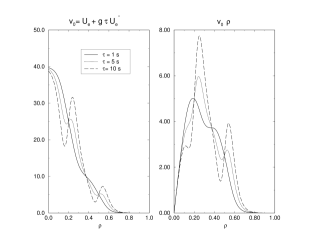
Figure 3: Left two panels: velocity isoclines (i.e points where accelerations vanish) for the homogeneous and stationary solution as a function of the local density $\rho$ for our model equations and the $U_{e}$ of the K³ model and the corresponding fundamental diagrams. All velocities are measured in ms^-1. Right two panels: dito but for the $U_{e}$ with a plateau.

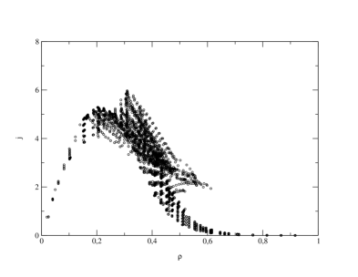
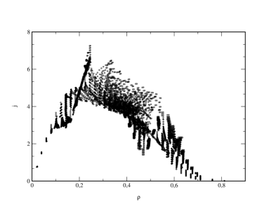
Figure 4: Shown are measured 1 minute averages of a set of simulations where the time scale $\tau$ has been scanned from 1 up to 10 s. The left panel results from using the conventional form of the safe velocity, for the right one the plateau function was used.

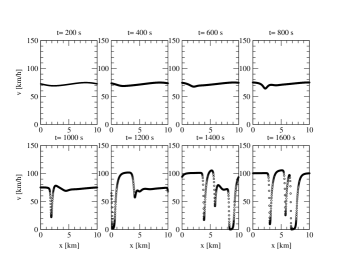
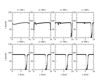
Figure 5: Emerging spontaneous breakdown of traffic flow in the unstable regime of our model ($\mu=50$ ms^-1 , $\tau=5$ s, $\rho_{in}=0.25$). The growing jam moves with $\approx 28$ km h^-1 backwards.

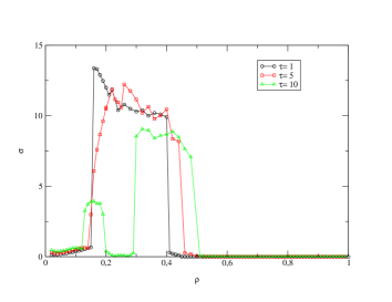
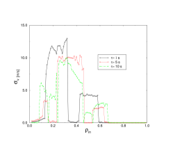
Figure 6: Velocity variance $\sigma_{v}$ for $\tau=1,5,10$ s as a function of the initial density for the conventional form of the safe velocity (left) and the plateau function (right).

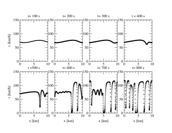
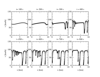
Figure 7: Formation of stop-and-go-waves out of nearly homogeneous initial conditions ($\rho_{in}=0.25,\mu=50$ ms${}^{-1},\tau=3$ s). For the left panel the conventional form of the safe velocity was used, the right panel corresponds to the plateau safe velocity.

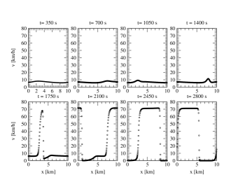
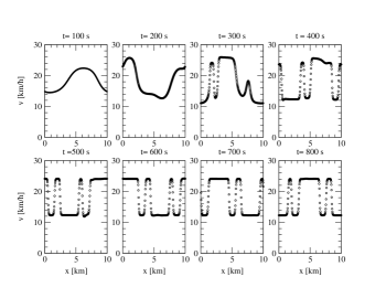
Figure 8: “Mesa-effect 1”: formation of velocity plateaus ($\rho_{in}=0.50,\mu=50$ ms${}^{-1},\tau=10$ s) for the conventional (left) and the plateau safe velocity (right).

Figure 9: Emerging spontaneous breakdown of traffic flow in the unstable regime of our model ($\rho_{in}=0.26$, $\mu=50$ ms${}^{-1},\tau=10$ s) with the plateau safe velocity. The use of the conventional safe velocity (not shown) results in a quick relaxation towards the homogeneous state.

Figure 10: Shown are comparisons of the $\sigma_{v}$ and $v_{0}$ as functions of $\rho$ for $\tau=10$ s (left) and $\tau=5$ s (right) for the case of the plateau function. Stability is encountered where $dv_{0}/d\rho$ is small, otherwise the flow is unstable.

Traffic modelling as well as traffic measurements have a long-standing tradition (e.g. Greenshields green35 , Lighthill and Whitham lighthill55 , Richards richards55 , Gazis et al. gazis61 , Treiterer treiterer74 , to name just a few). In recent years physicists working in this area have tried to interpret and formulate phenomena encountered in traffic flow in the language of non-linear dynamics (see, for example, the review of Kerner TGF99_kerner and many of the references cited therein). The measured real-world data reveal a tremendous amount of different phenomena many of which are also encountered in other non-linear systems.
To identify properties of our model equations we apply them to a closed one-lane road loop. The loop has a length of $L=10$ km and we prepare initial conditions close to a homogeneous state with density $\rho_{in}$ (i.e. same density and velocity everywhere). The system is slightly perturbed by a sinusoidal density perturbation of fixed maximum amplitude $\delta\rho=0.01$ and a wavelength equal to the loop length. The particles are initially distributed equidistantly, the weights $n_{i}$ are assigned according to (10) in order to reproduce the desired density distribution, and the velocities corresponding to $U_{e}(\rho)$ are used. All calculations are performed using 500 particles.
It is important to keep in mind that the results are only partly comparable to real world data since the latter may reflect the response of the non-linear system to external perturbations like on-ramps, accidents etc. which are not included in the model.
In the following the model parameter $\tau$, which determines the time scale on which the flow tries to adapt on $U_{e}$, is allowed to vary. This corresponds to a varying acceleration capability of the flow due to a changing vehicle composition (percentage trucks etc.). This parameter $\tau$ which is typically of the order of seconds controls a wide variety of different dynamical phenomena. A similar result has been found in IDM for a microscopic car-following model.

IV.1 Analysis of the Model Equations

IV.1.1 Fundamental diagram

The $x$-isocline, i.e. the locus of points in the $x-v$-plane for which $\frac{dx}{dt}=0$, is found from eq. (12) to be the abscissa. The velocity isocline, i.e. the $(x,v)$-points where the acceleration vanishes can be inferred from eq. (13). For the homogeneous and stationary solution one finds the isocline velocity $v_{0}$ as a function of $\rho$:

$$v_{0}(\rho)\equiv U_{e}(\rho)+g\tau U^{\prime\prime}_{e}(\rho).$$ (14)

Fixed-points of the flow, defined as intersections of the $x$- and $v$-isoclines, are thus expected only for densities above $\approx 0.6$, where $v_{0}$ approaches the abscissa, see Fig. 3. The flow of the homogeneous and stationary solution has no fixed point in a strict sense since $U^{\prime\prime}_{e}$ becomes extremely small at $\rho=1$, but does not vanish exactly. However, this could easily be changed by choosing another form of $U_{e}$. Fig. 3 shows these “force free velocities” $v_{0}$ (in the homogeneous and stationary limit) together with the “force free fundamental diagrams” (for $\tau=1,5,10$ s) for both investigated forms of $U_{e}$. We expect the fundamental diagrams (FD) found from the numerical analysis of the full equation set to be centered around these “force free fundamental diagrams”. While for the $U_{e}$ of the $K^{3}$-model the FD always (i.e. for $\tau=1,5,10$ s) exhibits a simple one-hump behaviour, eq. (8) leads to a one, two or three hump structure of the FD depending on the time constant $\tau$. That is why a stronger dependence of qualitative features on this constant may be expected for the plateau safe velocity. Note, however, that even with the conventional $U_{e}$ the “force free velocity” $v_{0}$ exhibits for $\tau=10$ s two additional extrema at intermediate densities (up to four with the plateau function). The implications of these additional extrema for the stability of the flow are discussed below.

IV.1.2 Stability

To get a preliminary idea about the stability regimes of the model it is appropriate to perform a linear stability analysis. By inserting (14) into the equations of motion we obtain equations that formally look like the equations of the $K^{3}$-model:

$$\dot{v}_{i}=\frac{v_{0}(\rho)-v_{i}}{\tau}-\frac{c_{0}^{2}}{\rho}\frac{\partial\rho}{\partial x}+\frac{\mu}{\rho}\frac{\partial^{2}v}{\partial x^{2}},$$ (15)

the role of $U_{e}$ now being played by $v_{0}$. Thus with the appropriate substitution the linear stability criterion of kerner93 can be used:

$$\frac{dv_{0}}{d\rho}<-\left[1+\left(\frac{2\pi}{L}\right)^{2}\frac{\mu\tau}{\rho}\right]\frac{c_{0}}{\rho}.$$ (16)

Thus we expect the flow to be linearly unstable in density regimes where the decline of $v_{0}$ with $\rho$ is steeper than a given threshold. Specifically, extrema of the $v_{0}(\rho)$ are (to linear order) stable and we therefore expect stable density regions embedded in unstable regimes.

IV.2 Simulation Results

The previous analytical considerations give a rough idea of what to expect, for a more complete analysis, however, we have to resort to a numerical treatment of the full equation set. In order to be able to distinguish the effects resulting from the additional term in the equations of motion from those coming from the form of $U_{e}$ we treat two cases separately: in the first case the conventional form of $U_{e}$ is used and in the second the effects due to a plateau in $U_{e}$ kerner93 are investigated.

IV.2.1 Conventional Form of $U_{e}$

To obtain a fundamental diagram (FD) comparable to measurements we chose a fixed site on our road loop. We determine averages over one minute in the following way: $\rho_{1m}=p^{-1}\sum_{i=1}^{p}\rho_{i}$ and $\j_{1m}=p^{-1}\sum_{i=1}^{p}\rho_{i}v_{i}$, where $p$ is the number of particles that have passed the reference point within the last minute. The thus calculated FD (Fig. 4, left panel) is, as expected, close to a superposition of the “force-free FDs”, for different values of $\tau$ see Fig. 3, left panel. As in real-world traffic data in the higher density regimes the flow is not an unambiguous function of $\rho$, but rather covers a surface given by the range of $\tau$ in the measured data. Note that many data points in the unstable regime (see below) exhibit substantially higher flows than expected from the ”force-free FDs” (see Fig. 3).
In certain density ranges the model shows instability with respect to jam formation from an initial slight perturbation. In this regime the initial perturbation of the homogeneous state grows and finally leads to a breakdown of the flow into a backward moving jam (Kerner refers to this state, where vehicles come in an extended region to a stop, as ”wide jam” (WJ) contrary to a ”narrow jam” (NJ) which basically consists only of its upstream and downstream fronts and vehicles do not, on average, come to a stop; PRL98 ). This phenomenon, widely known as ”jam out of nowhere”, is reproducible with several traffic flow models (e.g. kerner93 ; nagel92 ; krauss98 ). An example of a spontaneously forming WJ accompanied by two NJs is given in Fig. 5, left panel, for an initial density of $\rho_{in}=0.25$. It is interesting to note that the initial perturbation remains present in the system for approximately 15 minutes without noticeably growing in amplitude before the flow breaks down. As in reality the inflow front of the WJ is much steeper than the outflow front of the jam. Note the similarity with the jam formation process within the K³-model kerner93 .
To give a global idea in which density regimes congestion phenomena occur we show in Fig. 6, left panel, the velocity variance $\sigma_{v}=\sqrt{\frac{1}{N}\sum_{i}(v_{i}-\bar{v})^{2}}$ for given initial densities. The system is allowed to evolve from its initial state until $\sigma_{v}$ converges. If $\sigma_{v}$ has not converged after a very long time $T_{s}$ (= 10000 s) it is assumed that no stationary state ($\sigma_{v}\approx$ const) can be reached and $\sigma_{v}$ is taken at $T_{s}$. $N$ denotes the particle number and $\bar{v}$ the average particle velocity in the system. For low values of $\tau$ (1 and 5 s) the system shows spontaneous jam formation in a coherent density regime from $\sim 0.16$ to $\sim 0.5$, comparable to measured data. For $\tau=10$ s a stable regime at intermediate densities surrounded by unstable density regimes is encountered. This region corresponds to the two close extrema seen in Fig. 3, first panel.
Another widespread phenomenon is the formation of several jams following each other, so-called stop-and-go-waves. This phenomenon is also a solution of our model equations, see Fig. 7, left panel. The emerging pattern of very sharply localized perturbations is found in empirical traffic data as well (see Fig. 14, detector D7 in TGF99_kerner ).
A very interesting phenomenon happens towards the upper end of the instability range ($\rho_{in}\sim 0.5$). After the initial perturbation has remained present in the system for more than 20 minutes without growing substantially in amplitude, see Fig. 8, suddenly a sharp velocity spike appears at $t=1750$ s that broadens in the further evolution until the system has separated into two phases: a totally queued phase, where the velocity vanishes on a distance of several kilometers, and a homogeneous high velocity phase, both separated by a shock-like transition. We refer to these states with homogeneous velocity plateaus separated by shock fronts as Mesa states.

IV.2.2 $U_{e}$ with Plateau

The numerically determined fundamental diagrams for the case with plateau is shown in Fig. 4, right panel. The additional extrema expected from the ”force-free velocity” $v_{0}$ are visible in the data points. We therefore conclude that if a pronounced plateau in $U_{e}$ really does exist, additional extrema should appear in the measured fundamental diagrams, at least for flows with poor acceleration capabilities, i.e. large $\tau$’s.
Also with the plateau function the system shows spontaneous jam appearance. The formation of an isolated, stable WJ is displayed in Fig. refwidejam, right panel. With a change in the parameter $\tau$ (10 s rather than 5 s as in Fig. 5) one finds a more complicated pattern with one WJ that coexists for a long time with constantly emerging and disappearing NJs, see Fig. 9.
The global stability properties for the case with plateau are shown in Fig. 6, right panel. As expected from the linear stability analysis (see eq. (16) and Fig. 3, right panels) we find alternating regimes of stability and instability rather than one coherent density range where the flow is prone to instability. For low ($\rho\lesssim 0.1$) and very high density ($\rho\gtrsim 0.7$), initial perturbations decrease in amplitude, i.e. the system relaxes towards the homogeneous state. In between these density perturbations may grow and lead to spontaneous structure formation of the flow. The stable regions within unstable flow are found around densities for which $\frac{dv_{0}}{d\rho}=0$. This is displayed for two values of $\tau$ in Fig. 10.
The accelerations in the model were never found to exceed $\sim 4$ ms^-2 for negative and $\sim 1.5$ ms^-2 for positive signs and thus agree with accelerations from real-world traffic data (for both forms of $U_{e}$). For reasons of illustration Fig. 11 displays velocities and the corresponding accelerations at one time slice of a simulation ($\rho_{in}=0.25,\mu=50$ ms${}^{-1},\tau=3$ s) for $U_{e}$ according to eq. (8).

Figure 11: Velocities and accelerations in a violently congested state (480 s after simulation start, $\rho_{in}=0.25,\mu=50$ ms${}^{-1},\tau=3$ s). The encountered accelerations are always and everywhere in the range expected from experimental traffic data.

Also the plateau function allows for stop-and-go-waves, see Fig. 7, right panel. The shown evolution process is close to what Kerner PRL98 describes as general features of stop-and-go-waves: initiated by a local phase transition from free to synchronized flow, numerous well localized NJs emerge, move through the flow and begin to grow. One part of the NJs propagates in the downstream direction (see e.g. the perturbations located at $\sim 2$ km at $t=400$ s) while the rest (at $t=400$ s at $\sim 8$ km) move upstream. Once the first WJ has formed after approximately 500 s the NJs start to merge with it. This NJ-WJ merger process continues until a stationary pattern of three WJs has formed (at around 1000 s; not shown) which moves with constant velocity in upstream direction. The distance scale of the downstream fronts of these self-formed WJs is in excellent agreement with the experimental value of 2.5 - 5 km PRL98 .
We found for the conventional form of $U_{e}$ a separation into different homogeneous velocity phases that we called Mesa states. This feature is also present if the plateau function is used. In Fig. 8, right panel, the initial perturbation organizes itself into different platoons of homogeneous velocities. These platoons are separated by sharp, shock-like transitions and form a stationary pattern that moves along the loop without changing in shape.

Figure 12: ”Mesa-effect 2”: the composition of the flow (e.g. the fraction of trucks) plays a crucial role for the stability of the velocity plateaus ($\rho_{in}=0.50,\mu=50$ ms${}^{-1},\tau=12$ s). The same initial conditions for the plateau function do not lead to a behaviour that is qulitatively different from Fig. 8, left panel.

The relaxation term in eq. (6) plays a crucial role for the stabilisation of this pattern. If, for example, the relaxation time $\tau$ is increased (see Fig. 12) and thus the importance of the relaxation term is reduced, the system is not able to stabilize the velocity plateau. It seems to be aware of these states, but it is always heavily disturbed and never able to reach a stationary state. Again, the composition of the traffic flow plays via $\tau$ the crucial role for the emerging phenomena.

V Summary

Starting from the assumption that a safe velocity $U_{e}(\rho)$ exists towards which drivers want to relax by anticipating the density ahead of them, we motivate a set of equations for the temporal evolution of the mean flow velocity. The resulting partial differential equations possess a Navier-Stokes-like form, they extend the well-known macroscopic traffic flow equations of Kühne, Kerner and Konhäuser by an additional term proportional to the second derivative of $U_{e}(\rho)$. Motivated by recent empirical results, we explore, in addition to the new equation set, also the effects of a $U_{e}$-function that exhibits a plateau at intermediate densities. The results are compared to the use of a conventional form of $U_{e}$.
These fluid-like equations are solved using a Lagrangian particle scheme, that formulates density in terms of particle properties and evaluates first order derivatives analytically by means of cubic spline interpolation and second order derivatives by equidistant finite differencing of the splined quantities. The continuity equation is fulfilled automatically by construction. This method is able to follow the evolution of the (in some ranges physically unstable) traffic flow in a numerically stable way and to resolve emerging shock-fronts accurately without any spurious oscillations.
The presented model shows for both investigated forms of $U_{e}$ a large variety of phenomena that are well-known from real-world traffic data. For example, traffic flow is found to be unstable with respect to jam formation initiated by a subtle perturbation around the homogeneous state. As in reality, stable backward-moving wide jams as well as sharply localized narrow jams form. These latter ones move through the flow without leading to a full breakdown until they merge and form wide jams. The distance-scale of the downstream fronts of these self-formed wide jams is in excellent agreement with the empirical values. The encountered accelerations are in very good agreement with measured values. For the $U_{e}$ with plateau we also find states where a stable wide jam coexists with narrow jams that keep emerging and disappearing without ever leading to a breakdown of the flow, properties that are usually attributed to the elusive state of ”synchronized flow”. Another, striking phenomena is encountered that we call the ”Mesa-effect”: the flow may organize into a state, where platoons of high and low velocity follow each other, separated only by a very sharp, shock-like transition region. This pattern is found to be stationary, i.e. it moves forward without changing shape. One may speculate, that these mesa states are related to the minimum flow phase found in the work using the ASEP as a model for traffic flow popkov99 .
In other regions of parameter space the flow is never able to settle into a stationary state. Here wide jams and a multitude of emerging moving or disappearing narrow jams may coexist for a very long time. Again, it may be presumeded that in these cases the system displays deterministic chaos, however, we did not check this beyond any doubt.
The basic effect of the new interaction term is to make the ”force-free velocity”, which essentially determines the shape of the fundamental diagram, sensitive to the relaxation parameter $\tau$. For large values of $\tau$ additional extrema in the ”force-free flows” are introduced and a stability analysis shows that that the flows are stable against perturbations in the vicinity of these extrema. This leads to the emergence of alternating regimes of stability and instability, the details of which depend on the shape of $U_{e}$. We find that if a pronounced plateau in $U_{e}$ really does exist, it should appear in the measured fundamental diagrams, at least for flows with poor acceleration capabilities, i.e. large $\tau$’s.
The crucial parameter besides density which determines the dynamic evolution of the flow and all the related phenomena is the relaxation time $\tau$. Since this parameter governs the time scale on which the flow tries to adapt to the desired velocity $U_{e}$, we may interpret it as a measure for the flow composition (fraction of trucks etc.). It is this composition that determines whether/which structure formation takes place, whether the system relaxes into a homogeneous state, forms isolated wide jams or a multitude of interacting narrow jams.

To conclude, this work shows that a surprising richness of phenomena is encountered if one allows for a slight change of the underlying traffic flow equations. Further work is needed in order to extend the qualitative description undertaken in this work and to find more quantitative relationships between the traffic flow models and reality.

References

- (1) W. Benz, in The numerical Modelling of Nonlinear Stellar pulsations, Kluwer Academic Publishers, Dordrecht (1990)
- (2) D. C. Gazis, R. Herman, and R. W. Rothery, Nonlinear Follow–the–Leader Models of Traffic Flow, Oper. Res. 9 545 –567 (1961).
- (3) B. D. Greenshields, Studying Traffic Capacity by New Methods, Civil Engineering, 1935.
- (4) M. Treiber, A. Hennecke, and D. Helbing, Congested traffic states in empirical observations and microscopic simulations, Physical review E 62, 1805 – 1824 (2000).
- (5) B. S. Kerner and P. Konhäuser, Cluster effect in initially homogeneously traffic flow, Phys. Rev. E 48(4), 2335 (1993)
- (6) S. Krauß, P. Wagner and C. Gawron, Metastable states in a microscopic model of traffic flow, Phys. Rev. E 55, 5597–5605 (1997).
- (7) R. D. Kühne, Macroscopic Freeway Model for dense traffic, Proceedings of the 9th International Symposium on Transportation and Traffic Theory, p. 21 (1984).
- (8) M. J. Lighthill and G. B. Whitham, On kinematic waves: a Theory of Traffic on long crowded Roads, Proceedings of the Royal Society, A 229, 317 (1955)
- (9) K.Nagel and M. Schreckenberg, A cellular automaton model for freeway traffic, J.Physique I, 2:2221 (1992)
- (10) H.J. Payne, Models fro freeway traffic and control, Math. Models Pub. Sys., Simul. Council Proc., 28, 51 (1971)
- (11) V. Popkov and G. M. Schuetz, Steady state selection in driven diffusive systems with open boundaries, Europhys. Lett. 48, 257 (1999)
- (12) B.S. Kerner, Experimental features of Self-organisation in traffic Flow, Phys. Rev. Lett. 81, 3797 (1998)
- (13) P. I. Richards, Shock Waves on the Highway, Oper. Res. 3, 42–51 (1955).
- (14) S. Rosswog, P. Wagner, “Car-SPH”: A Lagrangian Particle Scheme for the Solution of the Macroscopic traffic Flow Equations, Traffic and Granular Flow 99, p. 401
- (15) B.S. Kerner, Phase transitions in traffic flow, Traffic and Granular Flow 99, p. 253
- (16) J. Treiterer, J. A. Myers, The Hysteresis Phenomenon in Traffic Flow, in D. J. Buckley (ed.), Proc. of the Sixth Intern. Symp. on Transportation and Traffic Theory, Elsevier 1974.