Chaotic Scattering of Microwaves

Abstract

In this paper we analyze a recent experiment conducted in an anechoic chamber, where the scattering of microwaves from an array of metallic cylinders was measured. This is a system which displays chaotic scattering in the short wave limit. The analysis of the experimental data is aimed at elucidating the effects of the underlying chaos. We describe a robust numerical method which provides the scattering matrix for any number of non overlapping reflecting cylinders. We use this method to calculate the scattering from one, two and three cylinders, and to compare the results in the numerical simulations with those obtained in the experiment. Both simulations and measurements validate the presented theory.

I Introduction

Scattering of electromagnetic waves in the microwave region is governed to a large extent by the underlying geometrical optics or ray dynamics, which provides the dynamical skeleton over which the residual interference and diffraction effects can be superimposed. In many instances, the ray dynamics is very complex, and it displays chaotic features which earns this phenomenon the name “chaotic scattering”. What makes the dynamics chaotic is that the scattering trajectories which come from infinity, are trapped for a long time within the interaction region before they escape to infinity. In the interaction domain, the motion is exponentially unstable, and therefore the outgoing trajectories hardly “remembers” the initial conditions. This results in very complex reaction patterns, fractal distributions, self similarity and other attributes which are typical of classical chaotic dynamics. As is well known, the complex patterns in dynamical systems are due to the existence of a “strange attractor” in phase space. In chaotic scattering, which is not a dissipative process, the “strange attractor” is replaced by a “strange repeller” which consists of all the trajectories which are trapped forever in the interaction domain. The complexity of the ray (or trajectory) dynamics manifests itself also in the corresponding wave phenomena (be it electromagnetic or acoustic waves or all possible de-Broglie –quantum– waves describing electrons, atoms or nuclei). The purpose of the present paper is to illustrate the importance of “chaotic scattering” in the context of electromagnetic wave physics.

The system which we studied in this work consists of three parallel metallic cylinders which scatter electromagnetic waves in the microwave region. This study has been performed by means of simulations and, what is more important, through measurements in the anechoic chamber of the European Microwave Signature Laboratory (EMSL) [1]. This system illustrates in an elegant and simple way the “generic” features of chaotic scattering. It is also a paradigm in the theoretical studies of this subject (see e.g., [2] [3],[4], [5] and references cited therein).

In the experiment, we measured the scattered fields in the TM mode (with the electric field parallel to the cylinders axis). The experimental set-up was planned such that one could neglect the coupling to the other polarization component. The antennas were in the far-field region of the cylinders (at a distance of about 10 m) and therefore the wavefront can be considered to be planar. The incidence is normal to the cylinders axis. This reduces the problem to the treatment of a two-dimensional (2-D) scalar field scattering of three cylinders in a planar geometry.

This paper is organized as follows. In Sect. II, we introduce the formulation of the problem and describe a robust numerical method which provides the scattering matrix for any number of non overlapping metallic cylinders. We use this method to calculate the scattering from one, two and three cylinders. Then, in Sect. III, we review the most important features which characterize the chaotic ray dynamics in the present system. The identification of the fingerprints of chaotic scattering of the rays in the actual experiments, where the scattering of waves of finite wavelengths are measured, is addressed in Sect. IV. For this purpose we make use of the Eikonel (semiclassical) approximation and propose a few correlation functions which are shown to depend explicitly on functions which characterize the chaotic dynamics of rays. In Sect. V, we turn to the description of the measurement set-up and the analysis of the experimental data. We compare the results in the numerical simulations with those obtained in the experiment. We show the actual correlation functions and compare them to the predictions of the short wave theory proposed. We end this work with a summary of our conclusions and a few suggestions for further experiments.

II Formulation of the Problem

Consider N parallel infinitely long conducting circular cylinders as shown in Fig. 1. The axes of the cylinders are parallel to the z-axis of a cylindrical coordinate system. The center of the $j$th cylinder of radius $a_{j}$ is located at ($R_{j},\phi_{j}$). A monochromatic plane wave with the electric field parallel to the axes of the cylinders (TM mode) impinges at an angle $\theta_{\rm{inc}}$. We assume a time dependence of the type $\exp(-iwt)$. The scattered field is scalar and must satisfy the planar wave equation

$$(\nabla^{2}+k^{2})\Psi=0$$ (1)

where $k$ denotes the frequency wavenumber. This equation is solved subject to Dirichlet boundary condition on the boundaries of the cylinders (i.e. the total tangential electric field vanishes on the surface of all cylinders). Thus

$$\Psi(\bf{r})|_{\bf{r}=\bf{r_{j}}}=0$$ (2)

where $\bf{r_{j}}$ is a point on the boundary of the cylinder $j$. At large observation distances, the solution may be decomposed into a summation of incoming and outgoing cylindrical waves as follows,

$$\Psi_{k,l}(\bf{r}) \simeq \frac{1}{(2\pi kr)^{1/2}}\times$$ (4)

$$\sum_{l^{\prime}=-\infty}^{\infty}\left[e^{-i[kr-(l^{\prime}\pi/2)-(\pi/4)]}\delta_{l,l^{\prime}}+S_{l,l^{\prime}}e^{i[kr-(l^{\prime}\pi/2)-(\pi/4)]}\right]e^{il^{\prime}\phi}$$

which is used as a definition of the scattering matrix $S$. This matrix contains all the information needed for a complete description of the scattering process and can be calculated exactly by making use of the KKR method [6]. The various matrix elements $S_{l,l^{\prime}}$ describe the scattering between states of different angular momenta $l$ and $l^{\prime}$. Because of flux conservation $S$ must be unitary.

Following the work of Gaspard and Rice [3] we proceed to the calculation of the $S$ matrix for the general case of $N$ non-overlapping cylinders. To this end, one uses the Green’s theorem in order to convert Eqs. (1) and (2) into an integral equation of the form

$$\int_{D}d^{2}r^{\prime}\left[\Psi_{k,l}(\bf{r}^{\prime})(\nabla_{\bf{r}^{\prime}}^{2}+k^{2})G_{0}({\bf r},{\bf r}^{\prime})-G_{0}(\bf{r},\bf{r}^{\prime})(\nabla_{\bf{r}^{\prime}}^{2}+k^{2})\Psi_{k,l}(\bf{r})\right]=$$ (5)

$$\oint_{\partial D}dr^{\prime}{\hat{n}(\bf{r}^{\prime})}\left[\Psi_{k,l}({\bf r}^{\prime})\nabla_{\bf{r}^{\prime}}G_{0}(\bf{r},\bf{r}^{\prime})-G_{0}(\bf{r},\bf{r}^{\prime})\nabla_{\bf{r}^{\prime}}\Psi_{k,l}({\bf r}^{\prime})\right].$$ (6)

Here, $D$ is the domain exterior to the cylinders but inside a circle with a boundary $\partial D_{\infty}$ which is large enough to enclose all the cylinders. $\partial D$ is the boundary of this domain, and the normal pointing outside is denoted by ${\hat{n}}(\bf{r}^{\prime})$. The boundary $\partial D$ of $D$ is the union of $\partial_{\infty}D$ and the boundaries of the $N-$cylinders and $\partial_{j}D,\,\,\,(j=1,\ldots,N)$. The free (outgoing) Green function is given by

$$G_{0}(\bf{r},\bf{r}^{\prime})=-\frac{i}{4}H_{0}^{(1)}(k|\bf{r}-\bf{r}^{\prime}|)$$ (7)

where $H_{0}^{(1)}$ is the zeroth-order Hankel function of the first kind.

Choosing $\bf{r}$ on the $j$ cylinder the first part of Eq. (5) vanishes and we get:

$$0=\sum_{i=1}^{N}\oint_{\partial_{j}D}dr^{\prime}{\hat{n}(\bf{r_{j}}^{\prime})}\left[G({\bf r_{j}},\bf{r_{j}}^{\prime})\nabla_{\bf{r}^{\prime}}\Psi_{k,l}(\bf{r_{j}}^{\prime})\right]$$ (8)

where the contour integral has $N+1$ parts. By calculating this integral [3], we obtain the gradient of the wavefunction at the cylinder boundaries as

$$A=CM^{-1}$$ (9)

where the matrix $A$ defines the gradient of the wave function

$${\hat{n}(\bf{r_{j}})}\nabla\Psi_{k,l}(\bf{r_{j}})=\sum_{m=-\infty}^{\infty}A_{ljm}e^{im\theta_{j}},\,\,\,\,l,m=0,\pm 1,\pm 2,\pm 3,...$$ (10)

and $\theta_{j}$ is the angular coordinate of the point $r_{j}$.

The matrix $M$ describes the multiple scattering between the $N$ cylinders and is found to be

$$M_{jmj^{\prime}m^{\prime}}=\delta_{mm^{\prime}}\delta_{jj^{\prime}}+(1-\delta_{j,j^{\prime}})\frac{a_{j}}{a_{j^{\prime}}}\frac{J_{m}(ka_{j})}{H_{m^{\prime}}^{(1)}(ka_{j^{\prime}})}H_{m-m^{\prime}}^{(1)}(kR_{j,j^{\prime}})\;\zeta_{j,j^{\prime}}(m,m^{\prime})$$ (11)

where $R_{j,j^{\prime}}=R_{j^{\prime},j}$ is the distance between the $j$ and $j^{\prime}$ cylinder, and $a_{j}$ is the radius of the $j$th cylinder. Note that $M$ has the structure of a KKR matrix and is the generalization of the results of Gaspard and Rice [3]. The matrix $\zeta$ is equal to

$$\zeta_{j,j^{\prime}}(m,m^{\prime}) = \exp\left[i(m\,\phi_{j^{\prime},j}-m^{\prime}(\phi_{j,j^{\prime}}-\pi))\right],$$ (12)

$$\zeta_{j,j^{\prime}}(m,m^{\prime}) = (-1)^{m-m^{\prime}}\zeta^{*}_{j^{\prime},j}(m^{\prime},m)$$ (13)

and contains–besides a phase factor–the angle $\alpha_{j^{\prime}j}$ of the ray from the center of the cylinder $j$ to the center of the cylinder $j^{\prime}$ as measured in the local coordinate system of cylinder $j$. In the simple case of one cylinder $M=\pi/2i$. Finally, the matrix $C$ is given by

$$C_{ljm}=\frac{2i}{\pi a_{j}}e^{il\Phi_{j}}\frac{J_{l-m}(kR^{j})}{H^{(1)}_{m}(ka_{j})}.$$ (14)

with $(R^{j},\Phi_{j})$ denoting the polar coordinates of the center of the $j$th cylinder as measured in the global coordinate system.

If we now take $\bf{r}$ outside the smallest circle which encloses all the cylinders, but inside the domain $D$, the first part of Eq. (5) provides $\Psi_{k,l}(\bf{r})$. We then obtain the $S$ matrix at large distance from the scatterer by propagating the wave function, whose gradient on the cylinders is now known. At the last stage of the calculation we use the asymptotic expansions of the Bessel functions at large distances $\bf{r}$ and the $S$ matrix is identified by comparing with the asymptotic expression (4). The final result reads,

$$S=I-iCM^{-1}D$$ (15)

with the matrix $D$ defined:

$$D_{ljm}=-\pi a_{j}J_{m-l}(kR^{j})J_{l}(ka_{j})e^{-im\Phi_{j}}.$$ (16)

The method presented above has the advantage that the calculation of the $S$ matrix is essentially reduced to the algebraic problem of inverting the matrix $M$ defined in Eq. (11). In principle, this matrix is infinite. However, in order to carry on with numerical calculations, we need to approximate it by a finite square matrix of dimension $L$. The integer $L$ is chosen in such a way that the truncated matrix is unitary to within the desired accuracy of the calculation [3].

The normalized scattered field is given in terms of the scattering matrix $S$ as

$$f(\theta_{\rm{inc}},\theta_{\rm{sct}};k)=\frac{e^{-i\pi/4}}{(2\pi k)^{1/2}}\sum_{l,l^{\prime}=-\infty}^{\infty}e^{-il(\theta_{\rm{inc}}-(\pi/2)}(S_{l,l^{\prime}}-\delta_{l,l^{\prime}})e^{il^{\prime}(\theta_{\rm{sct}}-(\pi/2)}.$$ (17)

where $\theta_{\rm{inc}}$ and $\theta_{\rm{sct}}$ denote the incidence and observation azimuth angles, respectively.

The 2-D bistatic radar cross section (RCS) is then simply computed as

$$\sigma_{\rm{bist}}(\theta_{\rm{inc}},\theta_{\rm{sct}};k)=\left|f(\theta_{\rm{inc}},\theta_{\rm{sct}};k)\right|^{2}.$$ (18)

The presented formulation takes multiple scattering to any order and is valid for any working frequency, provided that the number of cylindrical modes used in the scattering matrix $L$ is sufficiently large. In the next section, we will focus on the chaotic behavior of the scattered fields in high frequency limit.

III Ray Dynamics

Under the approximation of the geometrical optics, the electromagnetic scattering is governed by the simple law of specular reflection at the boundary of the cylinders. Given an arbitrary frame of reference, any incoming ray can be identified by its direction $\theta_{i}$ and by the nearest distance by which it approaches the origin - the impact parameter $b_{i}$. The impact parameter is proportional to the angular momentum $l_{i}=kb_{i}$ where $k$ is the wavenumber. In the domain of all possible initial rays $(\theta_{i},b_{i})$, there is a compact set of values for which the corresponding rays will impinge on one of the cylinders. An initial ray in this relevant set will undergo multiple reflections by the cylinders, until it is scattered away emerging as the outgoing ray $(\theta_{f},b_{f})$. The function $\theta_{f}(b_{i};\theta_{i})$ where $\theta_{i}$ is kept fixed and $b_{i}$ varies within the relevant set is called the deflection function.

For scattering on a single cylinder whose center is at the origin, we have

$$\theta_{f}(b_{i};\theta_{i})=\theta_{i}+2\arcsin{b_{i}}\ \ \ \rm{for}\ \ \ |b_{i}|\leq 1.$$ (19)

The cylindrical symmetry implies $b_{f}=b_{i}$, and the actual deflection $\theta_{f}-\theta_{i}$ is independent of $\theta_{i}$. Adding another cylinder has two important consequences- the cylindrical symmetry is broken, and multiple scattering becomes possible in the vicinity of the trapped orbit which runs along the line which connects the two centers of the cylinders. Note that a ray which starts at infinity, can approach the trapped ray arbitrarily closely, but it must finally emerge. The resulting deflection function cannot be calculated analytically. Its complex structure is shown in Fig. 2a. The complexity is due to the fact that the trapped orbit is unstable. (The instability emerges because the reflections are induced by concave mirrors). The longer the scattering orbits dwells next to it, the more rapid are the fluctuations in the deflection function. The concept of “dwell time” is essential for the following discussion and it will be properly defined for a general scattering ray (independently of the number of cylinders it may encounter). Consider a scattering ray coming from $\theta_{i},b_{i}$, and after $Q$ reflections it goes out with $\theta_{f},b_{f}$. Denote the reflection points on the various cylinders by $\vec{r}_{j}$, with $1\leq j\leq N$. Then the dwell time (measured in units of length) is defined as

$$\tau(\theta_{i},b_{i})={1\over c}\left\{\sum_{j=1}^{Q-1}|{\vec{r}}_{j+1}-{\vec{r}}_{j}|+{\vec{r}_{1}}\cdot{\vec{n}_{i}}-{\vec{r}_{Q}}\cdot{\vec{n}_{f}}\right\}.$$ (20)

Here, $c$ is the speed of light, ${\vec{n}_{i}}$ and ${\vec{n}_{f}}$ are unit vectors in the incoming and the outgoing directions. The last two terms above, remove the arbitrariness in the definition of the point at which the dwell-time stop-watch starts (and stops) to tick. Fig. 2b shows the dwell time which correspond to the deflection function for two cylinders. The correlation of the complexity of the deflection with the dwell time is evident.

To generate chaotic scattering, one needs at least one more cylinder, which should be placed such that no cylinder interrupts (shadows) the lines which connect the boundaries of its neighbors. In this case, there exists a Cantor set of trapped orbits which can be encoded by the following symbolic dynamics: Denote the three cylinders by the letters $A,B,C$. Then, to any infinite string of letters $\{X_{i}\}_{i=1}^{\infty}$, $X_{i}\in\{A,B,C\}$, with $X_{i}\neq X_{i+1}$ there corresponds an unstable trapped orbit. If the string is $N$ periodic $(X_{i}=X_{i+N})$ for all $i$, the trapped unstable orbit is periodic. This is the “strange repeller” which is responsible for the chaotic dynamics in our system: A ray which comes from infinity and is scattered by the three cylinders is affected by an infinite set of trapped orbits. It can dwell next to any of them for some time, and then, due to the intrinsic instability, it can either be trapped next to another member of the repeller, or scatter out. The resulting dynamics is much more complex than what we saw in the two cylinders system, and it has the following features:

• The deflection function is singular on a Cantor set of $b_{i}$ values, showing self similar structures which occur on all scales (see Fig. 3).

• The dwell time function is singular on a Cantor set of $b_{i}$ values, which is correlated with the singular, self similar structures observed in the deflection function (see Fig. 4).

• The deflection function displays also smooth sections, which are due to single scattering from the convex hull of the boundary. These trajectories correspond to short dwell times, and we shall refer to this component of the scattering system as “direct”.

• Excluding the direct component, the rest of the scattering dynamics is ergodic - any bundle of neighbor incident trajectories emerge with $(\theta_{f},b_{f})$ values which are uniformly distributed over the relevant set defined above.

• The distribution of dwell times is asymptotically exponential (see Fig. 5a)

  $$P_{\rm{dwell}}(\tau)\approx\gamma_{\tau}\exp(-{\tau\gamma_{\tau}})$$ (21)

  and

  $$\gamma_{\tau}=(1-d_{H})\lambda$$ (22)

  where $d_{H}$ is the Hausdorff dimension of the Cantor set of singular points on the $b_{i}$ axis, and $\lambda$ is the Lyapunov exponent which characterizes the instability of the strange repeller.

• The distribution of impact parameter transfers (defined as the difference between the final and the initial impact parameters) for the ergodic component is approximately uniform

  $$P_{\rm{impact}}(b)\approx\left\{\begin{array}[]{ll}{1\over D}&\mbox{if $|b|\leq D/2$}\\ 0&\mbox{otherwise}\end{array}\right.\ \ .$$ (25)

  $D$ is an effective diameter of the part of the scatterer which induces the ergodic scattering component (see Fig. 5b).

Much more can be written on the mathematics and physics of chaotic ray scattering. The interested reader can find more details and references in the articles cited above. The material presented above suffices for the purpose of the following discussion.

IV Correlation Functions – The Fingerprints of Chaotic Dynamics

The scattering amplitude $f(\theta_{1},\theta_{2};k)$ is the transition amplitude to scatter from $\theta_{1}$ to $\theta_{2}$ at a wavenumber $k$. In the Eikonel approximation the scattering amplitude can be expressed as a superposition of amplitudes. Each amplitude corresponds to a geometrical ray which is incoming from $\theta_{1}$ and is out-going in the direction $\theta_{2}$. These rays are identified in the following way. Consider the deflection function $\theta_{f}(b_{i};\theta_{i})$ where $\theta_{i}$ is fixed at the value of interest $\theta_{1}$ and one looks for the impact parameters $b_{i}^{s}$ which satisfy the equation

$$\theta_{2}=\theta_{f}(b_{i}^{s};\theta_{1}).$$ (26)

The geometrical rays which are incoming at $(b_{i}^{s},\theta_{1})$ emerge at $\theta_{2}$, and hence they correspond to the desired transition $\theta_{1}\rightarrow\theta_{2}$. Due to the fact that the deflection function oscillates wildly as a function of $b_{i}$, there is an infinite set of values $b_{i}^{s}$ which satisfies (26). The Eikonel approximation for the scattering amplitude is

$$f(\theta_{1},\theta_{2};k)\approx\left(2\pi k\right)^{-{1\over 2}}\sum_{s}\left[{\partial^{2}\tau(\theta_{1},\theta_{2})\over\partial\theta_{1}\partial\theta_{2}}\right]^{1\over 2}_{s}{\rm e}^{ik\tau(\theta_{1},\theta_{2})|_{s}+i\nu_{s}{\pi\over 2}}.$$ (27)

Here, the sum goes over all the rays which satisfy (26), and the dwell time for each ray (20) appears explicitly, and it is considered as a function of the parameters $\theta_{1},\theta_{2}$ which define the transition. The pre-exponential factors can be interpreted as the partial scattering amplitudes brought by the individual rays. As a matter of fact, the sum of their absolute squares is the cross section in the geometrical optics approximation. It is obtained by deleting from the Eikonel cross section all the terms which come from interferences of contributing amplitudes. The integers $\nu_{s}$ are the Maslov indices.

The scattering amplitude gets contributions not only from the multiply reflected rays, but also from the “direct” component of rays which scatter from the convex hull of the cylinders. The statistical treatment we propose is not applicable for this component, and we have to subtract it from the measured or calculated data. This is done using the following reasoning. The “direct” component corresponds to very short dwell times, and therefore its dependence on $k$ is very smooth. Therefore, if one subtract the $k$ smoothed scattering amplitude one remains with the desired statistical component. The smoothing is done over a $k$ interval of the size $\Delta k$ centered about $\bar{k}$. In the present case, the smoothing interval was taken to be the entire interval where the measurement was carried out. Thus, the “statistical” component of the scattering amplitude is

$$\tilde{f}(\theta_{1},\theta_{2};k)=f(\theta_{1},\theta_{2};k)-{1\over\Delta k}\int_{\bar{k}-\Delta k/2}^{\bar{k}+\Delta k/2}f(\theta_{1},\theta_{2};k){\rm d}k\ \ .$$ (28)

The $\tilde{f}(\theta_{1},\theta_{2};k)$ is the primary object of our statistical study. Its Fourier transform with respect to $k$ provides the spectrum of dwell-times for the rays which support the transition $\theta_{1}\rightarrow\theta_{2}$. When averaged over the incoming and outgoing directions, it should coincide with the expression (21) i.e.

$$\left<\left|\int dk\tilde{f}(\theta_{1},\theta_{2};k)e^{-ikc\tau}\right|^{2}\right>_{\theta_{1},\theta_{2}}\simeq e^{-\gamma_{\tau}\tau}.$$ (29)

A comparison between the experimental measurement and the classically expected exponential decay is shown in Fig. 6. The behavior is clearly exponential over some 7 decades. The slope of the curve is equal to $\gamma_{\tau}\approx 1.068\ ns^{-1}$, in reasonable agreement with the value $\gamma_{\tau}=0.95\ ns^{-1}$, calculated from the ray dynamics.

We will now define the angle averaged correlation function

$$C_{\theta}(\epsilon)=\int_{0}^{2\pi}{{\rm d}\alpha\over 2\pi}\left\langle\tilde{f}(\alpha,\alpha+\Delta\theta;k)\tilde{f}^{*}(\alpha+\epsilon,\alpha+\epsilon+\Delta\theta;k)\right\rangle_{k}\ .$$ (30)

Here, we consider a situation where the outgoing angle relative to the incoming direction $\Delta\theta$ is kept constant, and one correlates the scattering amplitudes for different orientations of the target. The $k$ averaging is the same as defined in (28). Using the Eikonel approximation (27) and the relations

$${\partial\tau(\theta_{1},\theta_{1})\over\partial\theta_{1}}=-b_{1}$$ (31)

$${\partial\tau(\theta_{1},\theta_{2})\over\partial\theta_{1}}=b_{2}$$ (32)

we can approximate the correlation function by

$$C_{\theta}(\epsilon)\approx\left\langle\int_{0}^{2\pi}{{\rm d}\alpha\over 2\pi}\sum_{s}p_{s}(\alpha,\Delta\theta){\rm e}^{-ik\epsilon(b^{(s)}_{1}-b^{(s)}_{2})}\right\rangle_{k}\ .$$ (33)

To derive this expression, we assumed that $\epsilon$ is small so that the phase differences can be approximated by the leading order in their Taylor expansion. Off-diagonal contributions are discarded due to the $k$ smoothing, and the pre-exponential factors are expressed in terms of the geometrical-optics partial cross sections

$$p_{s}(\alpha,\Delta\theta;k)=2\pi k\left|{\partial^{2}\tau(\theta_{1},\theta_{2})\over\partial\theta_{1}\partial\theta_{2}}\right|_{s}\ \ {\rm with}\ \ \theta_{1}=\alpha\ ;\ \theta_{2}=\alpha+\Delta\theta.$$ (34)

The sum is extended over all rays $s$. We can now collect together all the partial cross sections which are due to rays for which the impact parameter transfer $(b^{(s)}_{1}-b^{(s)}_{2})$ equals $b$

$$P_{impact}(b;k)=\sum_{s}\int_{0}^{2\pi}{{\rm d}\alpha\over 2\pi}\sum_{s}p_{s}(\alpha,\Delta\theta;k)\delta((b^{(s)}_{1}-b^{(s)}_{2})-b)$$ (35)

With this definition we get

$$C_{\theta}(\epsilon)\approx\left\langle\int_{-\infty}^{\infty}{{\rm d}bP_{impact}(b;k)\rm e}^{-i\epsilon kb}\right\rangle_{k}\ .$$ (36)

Since we subtracted away the “direct” contribution, we can use the ergodicity of the chaotic component and estimate $P(b)$ by the expression (25 ).

In a similar way we can define the cross correlation

$$X_{\theta}(\epsilon)=\\ \int_{0}^{2\pi}{{\rm d}\alpha\over 2\pi}\left\langle\tilde{f}(\alpha,\alpha+\Delta_{1}\theta;k)\tilde{f}^{*}(\alpha+\epsilon,\alpha+\epsilon+\Delta_{2}\theta;k)\right\rangle_{k}\ .$$ (37)

where, in contrast with (LABEL:corr1) we correlate scattering amplitudes measured at two different detector configurations. The rays which support the scattering in the two configurations are completely unrelated, and therefore we expect

$$X_{\theta}(\epsilon)=0.$$ (38)

Another useful correlation function can be defined by

$$C_{k}(\nu)=\\ \int_{0}^{2\pi}{{\rm d}\alpha\over 2\pi}\left\langle\tilde{f}(\alpha,\alpha+\Delta\theta;k+\frac{\nu}{2c})\tilde{f}^{*}(\alpha,\alpha+\Delta\theta;k-\frac{\nu}{2c})\right\rangle_{k}\ .$$ (39)

By repeating a similar argument as above, one can express $C_{k}(\xi)$ as a Fourier transform of the dwell time distribution

$$C_{k}(\nu)\approx\int_{-\infty}^{\infty}{{\rm d}\tau P_{dwell}(\tau)\rm e}^{-i\nu\tau}\ .$$ (40)

The dwell time distribution $P_{dwell}(\tau)$ was discussed above, and the expression (21) implies that the $|C_{k}(\nu)|^{2}$ is a Lorentzian with a width which is proportional to $\gamma_{\tau}$.

The two correlation functions obtained above are typical for scattering systems for which the resonances are overlapping and which display therefore Erickson type fluctuations [4]. One of the most important achievements of the theory of chaotic wave scattering was to recognize the fact that Erickson fluctuations are the hallmark of the underlying chaotic ray dynamics.

Several other correlation functions (e.g., Hanbury-Brown Twiss type correlations) can also be computed [4]. However, the measurement requires the use of two receiving antennas at close (angular) proximity. This experiment was not yet carried out.

V Measurement Description and Data Analysis

Before comparing our numerical simulations with the experimental measurements we shall give a short description of the experimental setup. The measurements were performed in the anechoic chamber of the European Microwave Signature Laboratory. This chamber has a hemispherical shape with a diameter of about $20$ m. It is equipped with two separate TX/RX antenna modules, which can be moved independently along a circular arch in a vertical plane, as well as $27$ receiving antennas which are on the uniformly distributed hemispherical dome. The range from the center of the chamber to all the antennas is the same: $9.56$ m. The system is fully polarimetric and operates in the stepped frequency mode.

The measurement set-up used in the experimental validation is shown is Fig. 7. The target (consisting of one, two or three identical copper cylinders of height $30$ cm and diameter $7.9$ cm) was placed on a rotating table whose axis of rotation is parallel to the axes of the cylinders. The center of gravity of the three-cylinders coincides with the rotation axis (vertical axis). Two different antenna configurations were used, and they are referred to as $T1$ and $T2$, with

• $T1$ configuration: TX at angle $89.5^{o}$; RX at angle $25.85^{o}$

• $T2$ configuration: TX at angle $-89.5^{o}$; RX at angle $25.85^{o}$.

For each configuration, the bistatic scattered fields complex amplitude was measured at $36$ equally spaced azimuth positions of the table at $10^{o}$ intervals. The data were sampled within the frequency interval $4-20$ GHz with a frequency step of $11.25$ MHz. The acquired data in the frequency domain were empty room subtracted and gated in the time domain in order to isolate the response of the cylinders from the residual antennas coupling and eventual spurious reflections in the chamber. Then a bistatic calibration using a metallic sphere of diameter $30$ cm placed at the focal point of the chamber, was applied in the HH and VV polarizations.

Some examples of experimental and numerical radar cross section vs. the frequency $\nu$ are shown in Figs. 8 and 9 for antenna configurations $T1$ and $T2$ and for one, two and three cylinders. As we see, the agreement of our numerical calculations with the experimental measurements is quite good within the entire frequency range.

We invested some effort to understand the deviations which appear for the $T1$ configuration at the higher frequency range. In principle, the scattering of a single cylinder should not depend on the table orientation. However, the experimental data show distinct periodic modulation with peak value of $\approx$ 15 %. This can only be explained as due to the finite geometry: the effective scattering angle does depend on the orientation since the cylinder was not placed at the center of the rotating table.

Finally, Fig. 10 shows the variations of the bistatic cross section for some specific values of frequency, when the azimuth position of the rotating table is varied. Again we are able to see a quite good agreement with the experimental results which lead us to the conclusion that our numerical calculations simulate quite well the experimental data.

We turn now to the statistical analysis of the scattering matrix. More specifically we calculate the various correlation functions defined in section IV in order to test the statistical predictions. Fig. 11 displays the functions $C_{\theta}(\epsilon)$ (LABEL:corr1) and $X_{\theta}(\epsilon)$ (LABEL:cross). The slight deviation of the cross correlation from the expected value $0$ is due to the fact that we perform a finite averaging over the frequencies. The autocorrelation function, however is consistent with Eq. (36).

Another interesting quantity we can evaluate is the energy correlation function $C_{k}(\chi)$ defined in Eq. (LABEL:corr2). From our semiclassical consideration, we expect it to have a Lorentzian form with half-width approximately equal to $\gamma_{\tau}$. Our results, reported in Fig. 12a are in agreement with the semiclassical prediction.

A direct consequence of the above result, and of the underlying ergodicity is that not only the amplitudes but also the cross sections show similar correlations in energy. We expect

$$C_{\sigma}(\nu)\equiv\frac{\left\langle\hat{\sigma}_{\rm{bist}}(k+\frac{\nu}{2c})\hat{\sigma}_{\rm{bist}}(k-\frac{\nu}{2c})\right\rangle_{k}}{\left\langle\hat{\sigma}_{\rm{bist}}^{2}(k)\right\rangle_{k}}\simeq\frac{1}{1+(\nu/\gamma_{\tau})^{2}}$$ (41)

where $\hat{\sigma}_{\rm{bist}}(k)\equiv\sigma_{\rm{bist}}(k)-\left\langle\sigma_{\rm{bist}}(k)\right\rangle_{k}$ is the fluctuating part of the cross section. Again, we calculate $C_{\sigma}(\nu)$ and recovered a satisfactory agreement with the semiclassical predictions. The results are shown in Fig. 12b.

VI Conclusions

We have presented an algorithm that takes multiple scattering to any order and we can use it to simulate any experimental configuration. We present results which show that chaotic scattering can be unambiguously identified in the experimental data. Moreover, the various theoretical simplifications which were assumed, as well as the finite angular resolution in the experiment, did not blur the signatures of the chaotic ray dynamics.

The main conclusion from the present calculations is that in the range of frequencies used in the experiments, the effects due to chaotic scattering are prominent in the present system and, in general in most systems in which electromagnetic radiation is scattered from metallic objects. The scattered radiation field is so complex, that it shows many features which would be typically attributed to a random field.

One may investigate the subject further by performing e.g., the measurements of the Hanburry-Brown Twiss effect, or by considering other scattering systems such as cavities (see [7]) or waveguide networks (see [8]). We also believe that the observations made here can be used, and should be taken into account when heterodyn electromagnetic radiation experiments analyzed.

List of Figures

lof

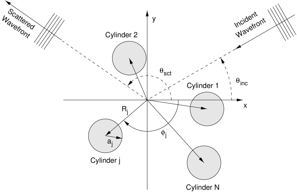
FIG. 1.: Geometry of the problem.

FIG. 2.: (a) The deflection function for the two cylinder system as a function of the impact parameter; (b) The corresponding dwell time as a function of the impact parameter

FIG. 3.: The deflection function for the three cylinder system as a function of the impact parameter. Three successive magnifications are shown, (the magnified domain is framed by dashes) and the fractal nature of the deflection function is obvious.

FIG. 4.: (a) The deflection function for the three cylinder for the entire range of impact parameter; (b) The corresponding dwell time exhibits singularities which are correlated with the self-similar structure observed in the deflection function.

FIG. 5.: (a) The probability distribution of the dwell times. The slope of the straight line is $0.95~{}\rm{ns}^{-1}$; (b) The distribution of impact parameters for the three cylinder system.

FIG. 6.: Fourier power spectrum of the measured $\tilde{f}(\theta_{1},\theta_{2};\nu)$ for the three cylinder system, averaged over $\theta_{1},\theta_{2}$ (dotted line). The best fit (bold line) and the the semi-classical prediction (dashed line) are shown.

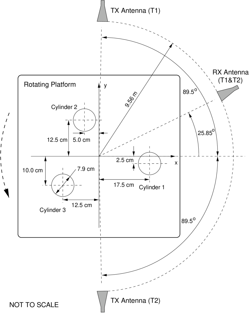
FIG. 7.: Sketch of the measurement set-up used in the experimental validation.

FIG. 8.: Experimental (circles) and numerical (stars) bistatic cross section vs. frequency for the $T1$ configuration.

FIG. 9.: Experimental (circles) and numerical (stars) bistatic cross section vs. frequency for the $T2$ configuration.

FIG. 10.: Experimental (circles) and numerical (stars) bistatic cross section vs. the azimuth position of the rotating platform $\alpha$ for the $T2$ configuration. The frequency is $10.485$ GHz.

FIG. 11.: Numerical calculation of the correlation functions $C_{\theta}(\epsilon)$ (solid line) and $X_{\theta}(\epsilon)$ (dashed line). The bold line correspond to the semiclassical prediction for $C_{\theta}(\epsilon)$. The antennas configuration is $T1$.

FIG. 12.: (a) The absolute value of $C_{k}(\nu)$ and (b) $C_{\sigma}(\nu)$. The solid lines correspond to the numerical results while the dashed one, to the semi-classical prediction for $\gamma_{\tau}=1.068~{}\rm{ns}^{-1}$. The bold dashed lines correspond to the experimental data. The antennas configuration is $T1$.

REFERENCES

- [1] A.J. Sieber, “The European Microwave Signature Laboratory”, EARSel Advances in Remote Sensing, Vol. 2, No. 1, pp. 195-204, January 1993.
- [2] B. Eckhardt, “Irregular Scattering of Vortex Pairs”, Europhys. Lett., Vol. 5, pp. 107-111, January 1987.
- [3] P. Gaspard and S. A. Rice, “Exact quantization of the scattering from a classically chaotic repeller”, J. Chem. Phys., Vol. 90, pp. 2255-2262, February 1989.
- [4] U. Smilansky In M.-J. Giannoni, A. Voros, and J. Zinn-Justin, editors, Proceedings of the 1989 Les Houches Summer School on “Chaos and Quantum Physics”, pp. 371-441. Elsevier Science Publishers B.V., Amsterdam, 1991.
- [5] A. Wirzba and M. Henseler, “A direct link between the quantum-mechanical and semiclassical determination of scattering resonances”, J. Phys. A: Math. Gen., Vol. 31, pp. 2155-2172, March 1998.
- [6] J. Korringa, “On the calculation of the energy of a Bloch wave in a metal”, Vol. 13, pp. 393-400, November 1947; F. S. Ham and B. Segall, “Energy Bands in Periodic Lattices- Green’s Function Method”, Phys. Review, Vol. 124, pp. 1786-1796, December 1961.
- [7] E. Doron, U. Smilansky and A. Frenkel, “Experimental demonstration of chaotic scattering of microwaves”, Phys. Rev. Lett., Vol. 65, pp. 3072-3075, December 1990.
- [8] T. Kottos and U. Smilansky, “Quantum Chaos on Graphs”, Phys. Rev. Lett., Vol. 79, pp. 4794-4797, December 1997.