![[Uncaptioned image]](/html/cond-mat/0110011/assets/x1.png)
![[Uncaptioned image]](/html/cond-mat/0110011/assets/x2.png)
Uni Essen and ITP preprint
cond-mat/0110011
September 30, 2001
Interacting Crumpled Manifolds
Henryk A. Pinnow1 and Kay Jörg Wiese1,2***Email: pinnow@theo-phys.uni-essen.de, wiese@itp.ucsb.edu
1 Fachbereich Physik, Universität Essen, 45117 Essen, Germany
2 ITP, Kohn Hall, University of California at Santa Barbara, CA 93106-4030, USA
In this article we study the effect of a -interaction on a polymerized membrane of arbitrary internal dimension . Depending on the dimensionality of membrane and embedding space, different physical scenarios are observed. We emphasize on the difference of polymers from membranes. For the latter, non-trivial contributions appear at the 2-loop level. We also exploit a “massive scheme” inspired by calculations in fixed dimensions for scalar field theories. Despite the fact that these calculations are only amenable numerically, we found that in the limit of each diagram can be evaluated analytically. This property extends in fact to any order in perturbation theory, allowing for a summation of all orders. This is a novel and quite surprising result. Finally, an attempt to go beyond is presented. Applications to the case of self-avoiding membranes are mentioned.
Keywords: polymer, polymerized membrane, renormalization group, exact resummation.
Submitted to Journal of Physics
1 Introduction
Interacting lines and more generally manifolds play an important role in many areas of modern physics. Examples of lines are self-avoiding polymers [?], vortex-lines in super-conductors [?], directed polymers in a disordered environment, also equivalent to surface growth [?], diffusion of particles and many more. Generalizing results to membranes often poses severe problems, but also new insight into physics. Recently, a lot of work has been devoted to self-avoiding membranes (see [?] for a review). Applications reach as far as high-energy physics, where strings and M-branes have been proposed as a general framework for unifying all fundamental interactions.

In this article, we focus on the statistical physics of systems without disorder. We think of situations like the binding and unbinding of a long chain as e.g. a polymer or a membrane on a wall or the wetting of an interface. More precisely, we study the interaction of a single freely fluctuating manifold with another non-fluctuating, fixed object. Depending on whether the interaction is attractive or repulsive, one can distinguish two different scenarios: One may either observe a delocalization transition from an attractive substrate as in wetting phenomena or steric repulsions by a fluctuating manifold. Both cases have in common that excluded volume effects become important. The situation for polymers or a 1-dimensional interface is relatively simple: One knows that in this case polymers interacting with a defect or a wall (excluding or not half of the space) as well as short-range critical wetting are in the same universality class [?,?]. For two-dimensional interfaces, the situation is more complicated, and a lot of effort has been spent to understand e.g. the delocalization transition [?,?,?,?,?,?,?,?]. Particularly, one is interested in critical wetting for the case of a short-ranged interaction potential. Then, it can not be approximated by a polynomial in the field and the conventional field-theoretic approach known from theory fails. This led to a couple of different ansätze [?,?,?,?,?], among others the functional renormalization group approach of [?,?].
Here we follow a different route: We start by constructing a systematic perturbative renormalization group treatment of the delocalization transition as well as the universal repulsive force exerted by a membrane on a point, line or more generally hyper-plane like defect. We therefore introduce a flexible “phantom” manifold of internal dimension . By introducing a -potential in a subspace of dimension , part of the embedding space (see fig. 1.2) we punish configurations crossing . Neglecting the effect of self-avoidance between distinct points within the fluctuating manifold, the free energy of a given configuration reads:
| (1.1) |
where is the position of monomer in embedding space , and denotes the -dimensional coordinate space of the manifold. In the case of a polymer this is simply the internal chain length. is the attractive or repulsive interaction, of dimension (in inverse length-units)
| (1.2) |
The interaction is naively relevant in the infrared for positive, and irrelevant for negative. In a perturbative treatment, is the natural expansion parameter. The situation is similar to self-avoiding membranes and thus (1.1) has been studied as a “toy-model” for the analysis of the renormalizability of the more complicated interaction in the generalized Edwards model for self-avoiding polymerized membranes [?,?,?]. It was shown to be renormalizable for arbitrary manifold dimensions [?,?]. This means that the large scale properties are universal, i.e. do neither depend on the regularization scheme used in these calculations, nor on the form of the contact interaction, as long as it is short-ranged. Universal quantities have thus been obtained to one-loop order. They are related, as we will show below, to the correction to scaling exponent , which as usually in critical phenomena contains deviations from the long-distance scaling behavior. Neglecting self-interactions, one has to distinguish between polymers, which are always crumpled and membranes, for which a highly folded high-temperature state is separated through a crumpling transition from an essentially flat low-temperature phase [?,?,?,?]. The effect of self-avoidance can also be taken into account [?,?,?,?,?]. It has been shown to lead as in the case of polymers to a swelling of the membrane and correspondingly to a non-trivial exponent for the radius of gyration [?,?]. However, it is not clear whether a fractal phase can be found in experiments or simulations. (See [?] for the latest simulations). In this work we will mostly neglect self-avoidance.
The aim of this article is two-fold: First, we present the necessary techniques to treat the model (1.1) beyond the leading order. We explicitly perform a two-loop calculation which gives the correction to scaling exponent at order . Specializing to membranes one finds that the 2-loop result naively diverges in the limit of . This is a problem of the -expansion, since there, diagrams have to be evaluated at , and taking implies causing the result to diverge. This motivated us to try a “massive scheme” in fixed dimension, i.e. finite . It turns out that the limit can then be taken and is regular. Even more, the -loop diagram, which for can only be calculated numerically, can now be evaluated analytically. This striking property even holds for higher orders, and we are able to give an explicit – quite simple – expression for the perturbation series. Then the whole series can be summed and the strong coupling limit analyzed. This is one of the very few cases where one can indeed obtain the exact relation between bare and renormalized coupling in the limit of , and thus the exact -function. This result does not depend on the explicit regularization and renormalization prescriptions, and is also obtained for a membrane of spherical or toroidal topology. In a final step, we lay the foundations for an expansion about . In contrast to the leading order, the first order corrections already depend on the cut-off procedure. We study one specific procedure, which turns out to reproduce results for polymers at leading order approximately, and even exactly in . Work is in progress to obtain a more systematic expansion about [?].
2 Model and physical observables
2.1 The model
We start from the manifold Hamiltonian (1.1). We split the total embedding space into and its orthogonal complement of dimension . Each points to a point , with and . The integration over the subspace is then trivial and gives
| (2.1) |
In the partition function
| (2.2) |
the contributions from the parallel and orthogonal components of factorize as
| (2.3) |
with
| (2.4) | |||||
| (2.5) | |||||
| (2.6) |
Since is trivial, we will only consider and shall drop the subscript ⟂ for notational simplicity. We keep in mind that cases with make sense, for instance a polymerized (non-selfavoiding) membrane interacting with a wall is described by (2.6) setting and .
Let us discuss (2.6) in more detail: The first term is the elastic energy of the manifold which is entropic in origin. We have scaled elasticity and temperature to unity. The second term models the interaction of the manifold with a single point at the origin in the external -dimensional space, but we remind that the physical interpretation may well be that of a line or surface. The coupling constant may either be positive (repulsive interaction) or negative (attractive interaction). We now give the dimensional analysis. In coordinate-space units, the engineering dimensions are
| (2.7) |
where
| (2.8) |
is an inverse length scale. The interaction is naively relevant for , i.e. with (see figure 2.2)
| (2.9) |
irrelevant for and marginal for . It has been shown [?,?] that the model is renormalizable for and . Results for negative are obtained via analytical continuation.

One can define the renormalized coupling as
| (2.10) |
where the normalization depends on the definition of the path-integral (but not on ) and is chosen such that
| (2.11) |
Universal quantities are obtained at fixed-points of the -function, which is defined as
| (2.12) |
The -function thus describes, how the effective coupling changes under scale transformations, while keeping the bare coupling fixed. Let us already anticipate the 1-loop result, which we derive later. It reads
| (2.13) |
where is the dimensionless renormalized coupling. Apart from the trivial solution, , the flow equation given by (2.12) and (2.13) has a non-trivial fixed point at the zero of the -function
| (2.14) |
We shall show below that the scaling behavior is described by the slope of the RG-function at the fixed point, which is universal as a consequence of renormalizabilty. The long-distance behavior is then governed by the -interaction as considered in our model (2.6), which is the most relevant operator at large scales. Let us now discuss possible physical situations (see fig. 2.4):
-
(a)
: The RG-flow has an infrared stable fixed point at and an IR-unstable fixed point at . The latter describes an unbinding transition whose critical properties are given by the non-interacting system, while the non-trivial IR stable fixed point determines the long-distance properties of the delocalized state, the long-range repulsive force exerted by the fluctuating manifold on the origin – which we remind may be a point, a line or a plane.
-
(b)
: Now, the long-distance behavior is Gaussian, while the unbinding transition occurs at some finite value of the attractive potential, , which corresponds to an infrared unstable fixed point of the -function. Below the manifold stays always attracted.
-
(c)
: This is the marginal situation, where the transition takes place at ; we expect logarithmic corrections to scaling.
Note that in the presence of an impenetrable wall constraining the configurational space strictly to half of the embedding space, the above considerations should still apply, when shifting the interaction strength appropriately. We shall discuss that in 2.3.
2.2 Repulsive force exerted by a membrane on a wall
Since we are mainly interested in the long-distance properties of membranes for which always (this is (a) on fig. 2.4), let us try to calculate the repulsive force exerted by the membrane on the origin in the case that this point is strictly forbidden. We will derive a universal expression for this force [?]. We need the (not normalized) membrane density at position
| (2.15) |
Since the -interaction also appears in , we can relate the density at the origin to the derivative of the partition function with respect to :
| (2.16) |
where is the renormalized or effective coupling defined in (2.10). Since is dimensionless, it depends on the dimensionless combination (and ) only. Using , we obtain
| (2.17) |
For the further considerations, it is sufficient to know the behavior of the -function close to the nontrivial zero. Expanding about , we have
| (2.18) |
Combining (2.16), (2.17) and (2.18), we get
| (2.19) |
The solution of this differential equation is
| (2.20) |
Using (2.17), this implies the scaling law
| (2.21) |
We now use this result to derive a scaling law for , with . In addition to (and ), depends on ; taking into account rotational symmetry and dimensionality, it depends on only through the dimensionless combination , with :
| (2.22) |
For , the most interesting limit is that of . Physically, this corresponds to strictly forbidding monomers to be at the origin. Therefore it is clear that this limit is well-behaved, and
| (2.23) |
is finite. In order to be consistent with (2.21) it has to obey a power law in the scaling regime
| (2.24) |
Comparing the -dependence of and , we obtain the exponent identity
| (2.25) |
Finally, from (2.24) we derive the repulsive force between the origin and the manifold
| (2.26) |
Note that to derive this result, has been set to 1. Reestablishing the temperature-dependence, we find
| (2.27) |
Also note that this argument gives at the Gaussian fixed point, which is necessary since for no force is excerted on the membrane.
2.3 Unbinding transition
Let us discuss the physical situation at the UV-stable fixed point in figure
2.4. The fixed point corresponds to a delocalization
transition of the manifold, which is at vanishing coupling for
and at some finite attractive coupling for
.
In the localized phase , correlation functions such as
and the associated correlation length
(in the -dimensional internal space) should be finite, as
well as the radius of gyration . Approaching the transition point
these quantities diverge as [?]
| (2.28) |
Since , the exponents and are related through
| (2.29) |
being the dimension of the field (2.7). To relate to , we first observe that depends only on and the membrane size , or its inverse . Writing as a function of the renormalized coupling and the scale , we thus have
| (2.30) | |||||
where the dimension-full factor has been factored from the dependence on the dimensionless renormalized coupling . Using that , this can be rewritten as
| (2.31) | |||||
The solution to the above equation is
| (2.32) |
This leads to the identification
| (2.33) |
Note that at the transition. Specializing to , we find
| (2.34) |
These exponents are also valid for the delocalization transition of a -dimensional interface from an attractive hard wall in -dimensional bulk space [?,?,?]. This can be understood as follows: The partition function of a fluctuating polymer interacting with a -defect at the boundary of a hard wall can be written as
| (2.35) |
where the sum runs over the number of contacts with the defect hyper-plane. denotes the contact energy, and is the constrained partition function of the free interface having exactly points of contact with the defect. The powers of only appear in the presence of an impenetrable defect and reflect the fact that all configurations in the presence of a hard wall can be obtained by flapping up those parts of the polymer which have penetrated the line (see figure 2.6). This accounts for a factor for each possible flap. Thus, the hard wall constraint translates into a shift in the binding energy according to
| (2.36) |
The delocalization transition occurring for at vanishing potential strength is shifted to an attractive interaction dependent on the temperature. Due to the correspondence (2.36) the exponents characterizing the transition remain unchanged.
3 Operator product expansion and one-loop result
The partition function of the model has been defined in (2.5). Analogously, we define the expectation value of an observable as (we denote for from now on)
| (3.1) |
Most physical observables can be derived from expectation values of general -point vertex operators like
| (3.2) |
Before we go on, let us make some changes in normalizations which will be helpful in the following. First, we rescale the field and the coupling constant according to
| (3.3) |
Second, we change the integration over internal coordinates to
| (3.4) |
being the volume of the -dimensional unit-sphere. Third, the normalization of the -distribution is changed to
| (3.5) |
with
| (3.6) |
The advantage of these normalizations is that
| (3.7) |
The model in the new normalizations now reads
| (3.8) |
and (due to the factor of in the above definition) the two-point correlator is
| (3.9) |
We now proceed with the calculation of physical observables. As an explicit example, let us consider the perturbation expansion of the -point vertex operator
| (3.10) |
where
| (3.11) |
This can be written as
| (3.12) |
where we have already integrated out a global translation of the field . The Gaussian average is:
| (3.13) |
The in (3.11) posses short distance singularities for . In order to analyze these singularities we will use the techniques of normal ordering and operator product expansion in the sequel. In our problem the procedure of normal ordering a vertex operator turns out to be quite simple: In any expectation value, we factorize out the contractions between the vertex operators. At one-loop order or equivalently at second order in (3.10) this means that
| (3.14) |
This can be understood as a definition of the normal ordered product . Note, that equality in the above equation is meant in the sense of
operators, that is when inserted into expectation values within the free
theory.
Let us now turn to an explicit derivation of the OPE of two
-interactions, i.e. we study (3.14) for small distances
. Since the short-distance singularities appear only in the
internal contractions, the normal ordered product in the r.h.s. of (3.14)
is regular for small distances and thus can be expanded
therein. We then project the resulting terms on the corresponding
operators. For that purpose we make a change in the momentum variables
according to
| (3.15) |
In internal space we change coordinates to the center of mass system:
| (3.16) |
Thus, the r.h.s. of (3.14) takes the form
| (3.17) |
Integration over yields the OPE of with :
| (3.18) | |||||
Restricting ourselves to the most relevant next to leading operators for internal dimension smaller than, but close to , the operator product expansion reads:
| (3.19) |
The OPE-coefficient in front of the leading operator, which is the -interaction itself, carries the leading short distance singularity. In the following we introduce some diagrammatic notation. Denoting we abbreviate the projection of two nearby -interactions on the -interaction itself as
| (3.20) |
We now analyze short-distance divergences of the perturbation expansion using the OPE in (3.18). Being interested in the leading scaling behavior, we drop all subdominant terms for , such that we only need the leading OPE-coefficient (3.20). The integral over the relative distance in is logarithmically divergent for . In order to define a counter term we use dimensional regularization, i.e. we set . The integral is then UV-convergent, but IR-divergent. An IR regulator or equivalently a subtraction scale has to be introduced to define the subtraction operation. Generally, we integrate over all distances bound by the inverse subtraction scale . The OPE-coefficient in (3.20) then reduces to a number as
| (3.21) |
Let us use the scheme of minimal subtraction (MS). The internal dimension of the membrane is fixed and (3.21) is expanded in a Laurent-series in , starting here at order . Denoting the term of order in by , the simple pole in (3.21) is
| (3.22) |
Of course, in this case, due to our normalizations, this is exact.
Let us rewrite the Hamiltonian in (2.6) in terms of the renormalized
dimensionless coupling . For perturbative calculations it is custom
to write
| (3.23) |
where is the renormalization factor, which is fixed by demanding that observables remain finite in the limit of . The Hamiltonian becomes
| (3.24) |
We find to one-loop order
| (3.25) |
There is no field-renormalization since the elastic part has also to describe the manifold far away from the origin, for which the interaction term can be neglected. Formally, of course, this follows from the OPE. The renormalization group -function is defined as
| (3.26) |
from what follows together with (3.23) that
| (3.27) |
To one-loop order we obtain from (3.27) and (3.25) as anticipated earlier
| (3.28) |
The long-distance behavior of the theory is governed by the IR–stable fixed point of the RG–flow. Fixed points are zeros of the –function:
| (3.29) |
In section 2.2, we had defined the correction-to-scaling exponent . It is obtained from the slope-function , defined as
| (3.30) |
The correction to scaling exponent is evaluated at the fixed points, and is found to be
| (3.31) |
Of course, this result is apart from the very existence of a fixed point rather trivial, since it is determined through the leading term of the -function, which is always . In order to obtain any non-trivial information from the perturbation series it is thus necessary to go beyond the leading order.
4 Two-loop calculation in a MS-scheme
4.1 Operator product expansion
Let us now continue with the calculation at the two-loop order. At each order of perturbation theory there is only one new diagram. At two-loop order this comes from three coalescing -interactions. Again, let us rewrite the product of the three vertex operators as its expectation value times the normal ordered product:
| (4.1) |
We use the following change of coordinates
| (4.9) |
As at 1-loop order, is free of divergences upon approaching the points , whereas the UV-divergence comes from the factor . The leading term is thus obtained upon setting in , dropping the gradient terms. Further shifting , we obtain
| (4.10) |
Integrating over , and yields the final result
where the OPE–coefficients are given by
| (4.12) | |||||
which contributes to the renormalization factor at two-loop order. The first subleading term is (denoting )
4.2 Numerical calculation in
Let us now turn to the explicit calculation of the second order contribution to the coupling constant renormalization. To two-loop order the renormalization group -factor for the coupling constant reads
| (4.14) | |||||
Note that this -factor can either be obtained from (2.10) and (3.23) or by expanding the perturbative series and checking that divergent contributions proportional to cancel.
The formula is arranged such that in the brackets the second order pole in cancels. This is, because to leading order in , the two-loop diagram factorizes into two one-loop diagrams. The combinatorial factor of is composed of a factor of 3 for the number of possible subdivergences, and a factor of for the nested integration: The subdivergence in the distance say only appears in the sector (i.e. part of the domain of integration) in which is smallest.
Let us define:
| (4.15) |
Let us already note that we will later calculate in a “massive” scheme in fixed dimension . In order to use the results derived here, we keep arbitrary instead of setting . We now want to derive an expression which can be integrated numerically. Since the bounds on the integrations in (4.15) are asymmetric (remind that in all 3 distances , , and are bounded by , whereas is an integral with two bounds only) we treat both terms separately. We start with the first one, which can be written as
| (4.16) |
The divergence when integrating over the global scale is eliminated by noting that . There remains of course the sub-divergences, which will be subtracted later by the counter-term. Applying this procedure to (4.16), we obtain
| (4.17) | |||||
Since the integral is symmetric in , , and , we can replace it by 3 times the first term. Introducing proper normalizations, an explicit representation for the measure and factoring out the explicit -dependence, we obtain
| (4.18) |
We also have to derive an expression for the counter-term. It can be written as
| (4.19) |
Using the same trick to derive w.r.t. the IR-regulator as above, we obtain
| (4.20) |
Using the technique of conformal mapping, which is presented in
appendix B,
both integrals above can be transformed into one having support in the
single sector defined through , (where here is set
to ). Analogously, we define sectors and
, as the subset of domains where respectively is
the longest distance. Note that the first term in (4.20) only has contributions
from and , while
the second can be restricted to and after
renaming into and into .
Performing explicitly the mapping of both and
onto one obtains
| (4.21) |
Combining the contributions from all sectors, we arrive at
| (4.22) |
Combining (4.18) and (4.22), we obtain an expression for the complete diagram
| (4.23) | |||||

|
This expression will also be used later in a massive scheme. Since here we are only interested in the -expansion, we take the limit of in the integrand. We have made the (non-trivial) check that the integrand remains a finite integrable function, which can be integrated numerically:
| (4.24) | |||||
Let us now proceed with the explicit numeric evaluation of (4.24). There are integrable singularities both in and . To disentangle them [?,?] we make a change of variables from Cartesian coordinates to radial and angular coordinates according to
| (4.25) |
such that
| (4.26) |
where the upper bounds of on and on is due to the bound of on and . We can further restrict integration to the half-sector with . In this sector, there remain singularities for small and small . The reader is invited to verify that they are eliminated by a second change of variables
The above method works for only. For , one has to
analytically continue the integration over in
(4.18). This can be done by partial integration, since the
integrand does not explicitly depend on but on
. To have no boundary
terms, one should partially integrate before mapping everything onto
the sector .
We have
explicitly checked consistency with the earlier used measure for . Note finally,
that in the special case of in (4.24) the integration measure
becomes a distribution reducing the integration measure to a line along
.
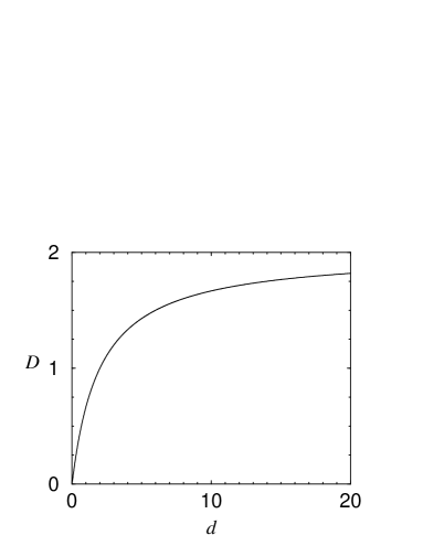
The diagram is shown on figure (4.4). It grows as for and exponentially for :
| (4.27) |
In the case of polymers it vanishes. The reason is that the diagrams factorize, and thus the 1-loop result is correct to all orders when working in an appropriate scheme. (See e.g. [?].)
4.3 RG-function and extrapolation
|
¿From (3.27) the renormalization -function in second order of perturbation theory reads
| (4.28) |
The long-distance behavior of the theory is governed by the IR–stable fixed point of the RG–flow. Fixed points are given by zeros of the –function:
| (4.29) |
The physically interesting nontrivial fixed point is the one that is next to zero. In an –expansion it reads:
| (4.30) |
The correction to scaling exponent at this fixed point is found in an -expansion to be
| (4.31) |
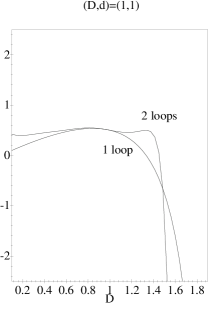
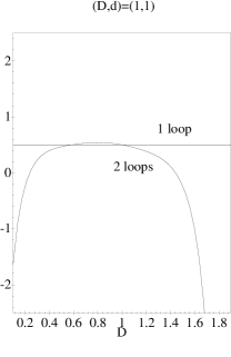
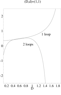
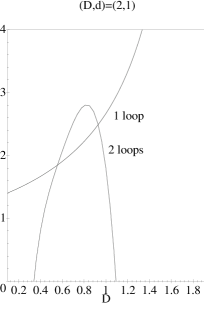
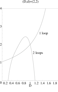
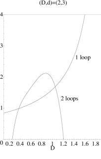
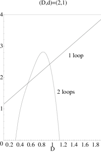
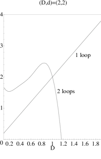
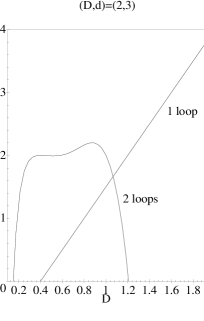
The question now arises of how to calculate for a given physical situation. The general strategy that we follow in the MS-scheme is that we make use of the freedom to choose any point on the critical line (2.4) around which to start our expansion [?,?]. To expand towards some physically interesting point we furthermore dispose of the freedom to follow any path starting on the curve . Since our expansion (4.31) is exact in but only of second order in , we can equally well expand it to second order in around any point on the critical curve. Now we can change our extrapolation path through an invertible transformation . One expresses and as functions of and and reexpands to second order in and around the point , where we recall that is defined such that . The aim is to find an optimal choice of variables . The guidelines for such a choice have been discussed in [?], where this procedure has been successfully applied to extrapolate results for the anomalous dimension of self-avoiding membranes. As a general rule, we “trust” most a result that is the least sensitive to the starting point of the extrapolation. Therefore, we would like to find a plateau for some suitable chosen variables . This procedure works well for polymers, or more generally for membranes with inner dimension close to 1. However it turns out that for membranes it works much less well than in the self-avoiding case: we could not find a plateau, but at best an extremum.
Some extrapolations are shown in the following figures (4.6, 4.8). We start with polymers interacting with a -wall corresponding to the point . (Note that for the interaction becomes relevant for polymers.) This can be seen on fig. 4.6. The values obtained from the plateaus appearing at the two-loop level are quite close to the exact value , known from the fact that the result in at one-loop is exact. From the latter it follows that it is best to use as extrapolation parameters and to stay in .
Let us now turn to the results obtained for extrapolated to points (fig. 4.20): The extrapolated value depends strongly on the starting-point on the critical line. We can identify a least sensitive value, which lies below , reflecting the -dependence of the two-loop diagram. We obtain identical results for different extrapolation paths. Note, that if we fix and perform an -expansion in as is commonly done [?], then, this corresponds to starting from . The -dependence of the extrapolated values is recovered in the massive scheme, which we discuss in the next section.
5 Calculation in fixed dimension: The massive scheme
5.1 Phantom manifolds
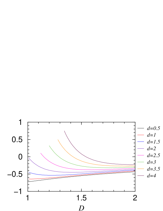
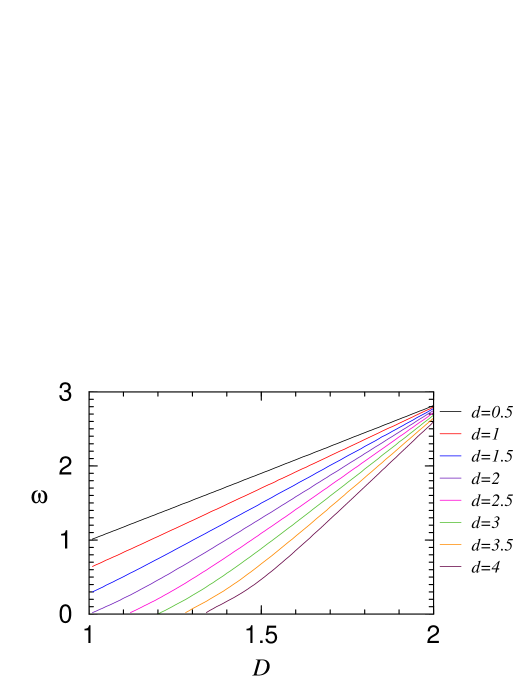
An alternative scheme to an -expansion is a calculation in fixed dimension. This way we hope to circumvent the difficulty that we faced when calculating the two-loop diagram in the previous section in the limit of : Since the diagram behaves like , it becomes large when the dimension of the embedding space is large. When working in an -expansion, and are related by and sending before imposes that . Thus one would like to work at finite , thus finite . The diagrams are UV-convergent for . They are cut-off in the infrared by a finite membrane size. Alternatively, we can use a “soft” IR cut-off, that is we introduce a chemical potential into the Hamiltonian and sum over all manifold sizes. For polymers this scheme corresponds to a “massive scheme” in an -symmetric, scalar -theory as can be seen via a de Gennes Laplace transformation on the component limit. (The correlator in momentum-space reads ) In the following we keep a hard IR regulator and calculate the two-loop diagram in fixed dimension. We use the analytical expression given in (4.23). For the numerical integration in we proceed as before. The result for different embedding dimensions is shown graphically on figure 5.2, where also some explicit values in the limit of are given. Note, that the exact factorization-property in the limit of is only valid in the MS-scheme or in a massive scheme with suitable soft cut-off as mentioned above. However, even the method is not tailored to capture that feature, the obtained value in the case of is not too far from the exact value . We expect that higher order terms would again reproduce the exact value of . Also note that results for membranes () are close to those from the -expansion, especially for small .
 0.5
-0.437
1
-0.410
1.5
-0.386
2
-0.358
2.5
-0.331
3
-0.299
3.5
-0.265
4
-0.229
0.5
-0.437
1
-0.410
1.5
-0.386
2
-0.358
2.5
-0.331
3
-0.299
3.5
-0.265
4
-0.229
 0.5
2.82
1
2.80
1.5
2.77
2
2.75
2.5
2.72
3
2.69
3.5
2.65
4
2.60
0.5
2.82
1
2.80
1.5
2.77
2
2.75
2.5
2.72
3
2.69
3.5
2.65
4
2.60
5.2 Self-avoiding membranes
Up to now we were considering a -dimensional polymerized “phantom” membrane interacting with a point-like impurity in -dimensional embedding space modeled through a -potential. The infinite fractal dimension of the free manifold was causing problems, and since all operators of the type , attain the same relevance in , it is not clear whether the model will break down. Physically, the problem is much better defined for self-avoiding membranes. From field-theoretical calculations, which have recently been refined up to two-loop [?,?], we know that two-dimensional self-avoiding manifolds embedded in three dimensional space have an anomalous dimension of . We now try to overcome the problem of an infinite Hausdorff-dimension by a crude simplification: We approximate the self-avoiding manifold by a Gaussian theory with the same scaling dimension, that is a Hamiltonian of the type [?]
| (5.1) |
where
as before providing the two-point correlator in our normalizations:
| (5.2) |
The scaling dimension is
| (5.3) |
We recover (3.9) by setting , but the model can be continued analytically to any real value of , with . Setting
| (5.4) |
we get a Gaussian manifold with identical scaling dimension as obtained for self-avoiding crumpled membranes at two-loop. The critical embedding dimension of the interaction then reads
| (5.5) |
that is the interacting is relevant in . For membranes . All operators of the type are at least naively irrelevant for , as
| (5.6) |
and the corresponding coupling has in inverse length units the dimension
| (5.7) |
We may repeat the calculation in the massive scheme setting the free scaling
dimension and . The result is shown in table
(5.2).
Let us stress that this method can not be turned into a systematic expansion,
since perturbation theory neglects all effects of the non-Gaussian nature of
the nontrivial crumpled state. We only know that for the
Gaussian variational approximation for the Hamiltonian, i.e. (5.1)
becomes exact [?,?,?].
|
6 Summation of the perturbation series in the limit
In the last section we introduced a “massive” scheme allowing to perform the renormalization procedure in fixed dimension. As can be seen in figures 5.2 and 5.4, the limit can be taken in the 2-loop diagram and is smooth. Surprisingly, this limit can be calculated analytically: Setting in (4.23), the integrand becomes constant, and thus trivial to calculate. This is a striking property. Even more, if we slightly modify the regularization prescription, this property holds to all loop orders in perturbation theory. Below, we will give an analytic expression for the complete perturbation series, which allows for analyzing the strong coupling limit. Furthermore, we show how corrections in can be incorporated. We will see that only the latter depend on the explicit cut-off procedure, a point which will be further clarified below. As a non-trivial check, when extrapolating back to polymers (), the corresponding result for is approximately reproduced.
6.1 -loop order
In order to calculate the –loop contribution to the perturbation theory we need the SDE of contact interactions. The normal ordered product of the corresponding vertex operators reads
| (6.1) |
We choose as root in the renormalization procedure (for the precise definition, see below) and therefore to integrate over in order to obtain the -distribution (or its derivative), onto which to project. We thus shift
and rewrite the quadratic form in (6.1) as
(6.1) then becomes (up to subdominant terms111Here we argue in terms of an OPE. Note that in order to make these arguments rigorous, one should ask of whether these terms affect the effective action at constant background-field. This is not the case, since then . involving spatial derivatives of )
and the integration over produces the -interaction and its derivatives; the latter come from the first term in (LABEL:6.2.a). They are subdominant and thus will be dropped. We abbreviate the quadratic form in (LABEL:6.2.a) as , where the matrix elements are
| (6.4) |
Integrating out the momenta yields the operator product expansion of contact interactions as
| (6.5) | |||||
6.2 The limit and -expansion
Whereas (6.5) is still completely general, we now want to study the limit as well as perturbations above it. We start by remarking that the matrix may be expanded in powers of :
| (6.6) |
where
| (6.7) |
. Then,
| (6.8) | |||||
where denotes the inverse matrix to . Let us expand the OPE-coefficient in (6.5) up to second order in . Expanding first the logarithm,
and inserting into (6.8) one arrives at
The zeroth order is . In order to proceed we need the latter and the inverse matrix . Let us first calculate the determinant. From (6.6) we have
| (6.20) | |||||
| (6.24) |
being the projector onto . Denoting by dim Im(P) the dimension of the space onto which projects one has the general formula:
Since here , we find
| (6.25) |
The inverse matrix of can be inferred from the ansatz
Since is a projector and this implies
Therefore, and
| (6.26) |
To obtain the first order contribution in from eq. (6.8) we only need , which reads
| (6.27) |
The trace of (6.27) can easily be performed, with the result
| (6.28) |
In order to factorize the integrals as much as possible, we found it convenient to modify the regularization prescription (3.21). In each order of perturbation theory we have to integrate the expression (6.5) over internal distances. These integrals have to be regularized in the infrared through an appropriate IR cut-off. In the preceding sections we have cut off the integrals such that all relative distances between internal points were smaller than . In the following we replace this by the demand that all distances from the fixed, but arbitrarily chosen point , the root of the subtraction prescription, are bounded by . Other distances are not restricted (see fig. 6.2). Alternatively, one could calculate on a closed manifold of finite size. Of course, then the correlator has to be modified. Work is in progress to implement this procedure, which has the advantage of being more systematic [?].

To simplify the calculations, we further introduce the following notation:
| (6.29) |
with new normalization
| (6.30) |
which is chosen such that the overbar can be thought of as an averaging procedure, and especially
| (6.31) |
Thanks to our regularization prescription the integral of (6.28) over internal points can be replaced by (for the integration measure ) times
| (6.32) | |||||
Introducing a diagrammatic notation
| (6.33) |
and
| (6.34) |
the -loop integral reads up to first order in
| (6.35) | |||||
We now turn to an explicit calculation of the diagrams. To first order in we have two contributions. The first (6.33) is
| (6.36) |
The second diagram (6.34) is
where we have put vectors to stress that is not a scalar. It suffices to evaluate this in . We find
| (6.37) |
Combining (6.35), (6.36) and (6.37) we finally obtain for the renormalized coupling up to first order in222The expression in parenthesis is the inverse renormalization -factor which relates the bare coupling to the renormalized coupling according to . :
| (6.38) | |||||
This can also be written as
| (6.39) | |||||
Absorbing a factor of both in and and defining the dimensionless coupling , we obtain the final result
| (6.40) | |||||
This formula is the starting point for further analysis in the subsequent sections.
6.3 Asymptotic behavior of the series
In the following we are interested in the limit of large (strong repulsion), which also is the scaling behavior of infinitely large membranes. We therefore need an analytical expression for sums like (6.40) in the limit of large . An example is the leading order expression
| (6.41) |
For the following analysis we need an integral representation of the above series. We claim that for all
| (6.42) |
This can be proven as follows:
This integral-representation is not the most practical for our purpose. It is better to set which yields
| (6.43) |
This formula is already very useful for some purposes. It is still advantageous to make a second variable-transformation , yielding
| (6.44) |
Finally we remark that we usually have the following combination
| (6.45) |
It satisfies the following simple recursion relation, which is helpful to calculate the -function:
| (6.46) |
From (6.42) for all and the behavior for large is obtained by expanding for small
| (6.47) | |||||
The result is
| (6.48) |
For later reference, we note a list of useful formulas ( is the Euler-constant)
| (6.49) | |||||
| (6.50) | |||||
Note that with the above notations, the relation (6.40) expressing as a function of becomes
| (6.52) |
In the next two sections we shall present two formalisms which give results for at next to leading order. It will turn out that the results catch qualitatively correctly the cross-over to ; however they differ in the numerical values. This is a reflection of the fact that the -expansion is not systematic. We expect that working on a manifold of finite size and using the exact correlation function on this manifold would lead to a systematic expansion. Work is in progress [?] to check this hypothesis.
6.4 The RG-functions in the bare coupling
The renormalization group -function is defined as
| (6.53) |
Since it is hard to invert the function , it is advantageous to study as function of the bare coupling
| (6.54) |
To first order in , we find from (6.52) using (6.46)
| (6.55) |
Inserting the asymptotic expansions from the last section, this becomes
| (6.56) |
where omitted terms have either one more power of or . As shown in section 2, universal properties are given by the correction to scaling exponent , reading
| (6.57) |
Let us first study . and are plotted on figure 6.4. We see that for the -function becomes 0 for . For , has no zero, but the flow of is still to infinity.
In both cases is given by . Taking only the leading term in the -expansion of , is given by
| (6.58) |
Let us now take into account the first order in . Then the fixed point of (6.56) is at the finite value
| (6.59) |
Next, when trying to calculate , we face the following problem: Since we truncated the series for at order one in , does not vanish at the fixed point, i.e. the zero of . This might lead to the conclusion that is always , an absurd result. However since this is a consequence of the truncation of the series, we follow the strategy also to expand the denominator of in powers of . From (6.55) and (6.57) we obtain:
| (6.60) | |||||
Inserting the asymptotic series, we find
| (6.61) |
Inserting the fixed point (6.59), we arrive at
| (6.62) |
This should be checked against the exact result in , which reads
| (6.63) |
Thus for our resummation-procedure gives the exact and for an approximative result. Before analyzing the validity of the procedure, let us turn to the second scheme, namely the calculation in the renormalized coupling.
6.5 Calculation in the renormalized coupling
We start from given in (6.52). For large this can be approximated by
| (6.64) |
where we only retained the leading term from each series. Also note that this formula is only valid for . For additional additive constants have to be added. Using (6.64), we can write as a function of . To first order in , this reads
| (6.65) |
We now write the -function in terms of . Starting from (6.56) we obtain
| (6.66) |
Fixed points are at the zeros of the -function. The non-trivial one is at
| (6.67) |
The correction to scaling exponent is simply obtained by evaluating the derivative of with respect to at the fixed point. In terms of this is
| (6.68) | |||||
Inserting the fixed point from (6.67) we find
| (6.69) |
Again, this is quite close to the exact result in , and in effect exact in and .
Let us finally point out that in the limit the true asymptotic behavior of the function in terms of the renormalized coupling is obtained from the completely summed series (6.41) leading to (6.66) for large . Conversely, if one tries to invert (6.41) and truncates it taking only a finite number of orders into account, it is at least possible to reach the asymptotic regime – however, for large enough the truncated function wildly oscillates and thus strongly deviates from the true behavior. In figure (6.6) the Pade-resummed truncated function up to order in is compared with the exact, asymptotic flow-function. One notices that the truncated -function eventhough improved throuh a Pade-Resummation hardly gets into touch with the asymptotic regime. The same applies to the slope-function , which is not shown in fig. (6.6).
Note that the above arguments suggest quite intuitively the behavior of the exact -function in . Whereas for , the -function is a parabola, and for it decays like a power-law for large at least as long as , the -function for values of between these two extremes should cut the axes at a finite value of , which for wanders off to infinity, thus by continuity forcing the exponent to go to 0 for .

6.6 An instructive case:
Setting in the leading order series (6.41) allows for a simple analytic expression for as a function of and its inversion
| (6.70) | |||||
| (6.71) |
This gives
| (6.72) | |||||
| (6.73) |
Fixed points are and with and . Note that the latter result is an artifact of .
7 Discussion and conclusion
In this article, we have discussed the perturbation expansion of a -dimensional elastic manifold interacting via a -interaction with a fixed point in embedding space. This calculation can be done exactly for , but becomes non-trivial for . Interestingly and quite surprisingly, it simplifies considerably in the limit of , if one decides to work at finite . In that limit we were able to obtain an explicit expression for the renormalized coupling as function of the bare one, in terms of a non-trivial series. Analysis of this series shows that the fixed point lies at infinity in the bare coupling, a limit in which we were able to derive an asymptotic expansion for the renormalized coupling as a function of the bare one. This yields a vanishing exponent in the limit of . Also it is important to note that this result is completely independent of the regularization procedure. This does no longer hold true beyond the leading order, which should be accessible to an expansion in . We here constructed its first order in a specific regularization scheme. While this reproduces qualitatively correctly the known results in (and even exactly for ), it also shows by its dependence on the renormalization scheme (here working with the -function either in terms of the renormalized or bare coupling) that this expansion in is not systematic. Even though experience with this new kind of expansion is still lacking, this is likely to be caused by the use of a hard cutoff in position space while working with the correlator of an infinite membrane. It seems that only in an -expansion this procedure is systematic. Work is in progress [?] to study the model on a sphere or torus of finite size, such that no further infrared cutoff is necessary. This should lead to exact results beyond the leading order and provide for the crossover between polymers and membranes.
While results for the pinning problem are interesting in its own, the main motivation is certainly to obtain a better understanding of self-avoiding polymerized membranes. This model is well-behaved physically, since its fractal dimension is bounded by the dimension of the embedding space . Preliminary studies [?] indicate that this problem can also be attacked by the methods developed in this article. This would be very welcome to check the 2-loop calculations [?,?] and the large-order behavior [?] on one side and numerical results (e.g. [?]) on the other.
Appendix A Universal - repulsion law for polymers
We have shown in section 2.2 by a scaling argument that as long as , the restricted partition function of a manifold pinned at one of its internal points scales as , with the contact-exponent given by (2.25). It is instructive to prove this for the special case of polymers in . According to (2.1) and (2.6) this corresponds to a polymer in -space interacting with a -potential on a plane.
Let us start from the (bulk) polymer propagator being defined as the conditional probability of finding the internal point at the position when starting in at . The propagator can be written as a functional integral for a restricted partition function of the free chain according to
| (A.1) | |||||
The propagator (A.1) posesses the Markov property
| (A.2) |
In the following we are interested in the restricted partition function (A.1) in presence of a short-range interaction modeled through a -potential, which is situated at the origin of the embedding space. The restricted partition function in the presence of the interaction will be denoted by . We consider the case, where the chain is fixed at its ends, such that and . We furthermore switch to a grand-canonical ensemble and denote
| (A.3) |
being some chemical potential. can be expanded in a perturbation series in the coupling according to
| (A.4) |
The are
| (A.5) | |||||
where we have used that after integration over , the integrals factorize; we further have defined
| (A.6) | |||||
In the integration over the momenta in (A.6) leads to
| (A.7) |
Let us now lock at what terms appear in the -th order coefficient in (A.5): From the initial point of the chain a factor is contributed, while the final point is coming up with . Furthermore, the internal points give powers of , where
| (A.8) |
The -coefficient is special: Clearly, one has
| (A.9) |
Inserting (A.8)-(A.9) into (A.5) we obtain for (A.4):
| (A.10) | |||||
The limit of can be taken and leaves us with the beautiful result
| (A.11) |
This is the propagator of a scalar field with Dirichlet boundary conditions. It has applications when studying critical phenomena of e.g. an Ising magnet in half-space [?,?]. Performing the inverse Laplace-transformation of (A.11) we arrive at
| (A.12) |
We conclude that a - potential acting in a
hyper-plane suppresses all configurations which penetrate or touch it,
when taking its amplitude to infinity.
Finally, in order to prove the universal repulsion law,
we start from (A.12) and
integrate over all final positions :
| (A.13) |
erf denoting the error function. For small arguments we have
| (A.14) |
Furthermore, denotes the restricted partition function of a chain pinned at one of its ends in . To obtain in (2.23) we have to evaluate:
| (A.15) |
according to (A.14) in the scaling regime . We thus find that , which confirms (2.25) for and . The above proof can be extended to arbitrary dimensions , where for polymers. Then, .
It would be nice to make the same arguments for membranes. However, the proof is based on a drastic simplification, which only occurs in and shows up in the factorizability of loop diagrams as in (A.5). This has no extension to manifolds of internal dimension .
Appendix B Conformal mapping of the sectors
In order to calculate the two-loop diagram efficiently, one wants to
write it as an integral over a finite domain only. To do so we need the technique of conformal
mapping of the sectors, which also serves for analytically continuing the
measure of integration to internal dimensions . This technique has
been extensively used and well documented in the context of self-avoiding tethered membranes
[?,?,?], but we repeat the
presentation here for completeness.
Generally, in evaluating the three-point divergences we need to
integrate over some domain in the upper half-plane (see
4.18). The measure of integration reads
| (B.1) |
and the integrand is a function of the three distances and between the points , and , given explicitly by (see fig. B.2)
| (B.2) |
In our problem is homogeneous, of degree , but not necessarily symmetric:
| (B.3) |
Let us now explicitly show, how sectors can be mapped onto each other. Specializing to the mapping we choose a coordinate system as given in figure (B.2). The mapping is mediated by a special conformal transformation, the inversion with respect to the circle around and radius . In complex coordinates this is ( is the complex conjugate of )
| (B.4) |
such that
| (B.15) |
This change of coordinates gives a Jacobian for the measure (B.1)
| (B.16) |
It can easily be seen that the mapping is one to one: First, be , that is and . Then,
| (B.17) |
and
| (B.18) |
Since , . Second, for the inverse mapping, is checked as follows:
| (B.19) |
since
and
| (B.20) |
Since and , . Finally, let us look at how the whole integral transforms. First inserting the transformed variables including the Jacobian (B.16) and second using the homogeneity (B.3), we arrive at
| (B.21) |
Let us restate the above calculation in a completely geometric interpretation as sketched in the figure. The mapping consists of two steps:
-
•
The rescaling with respect to by a factor which maps onto and onto . (B.3) implies that is changed by a factor .
-
•
A mirror operation, which maps onto and onto , leaving invariant the origin . This operation is a permutation of the first two arguments of .
The mapping corresponds to the special conformal
transformation (B.4).
Analogously, we find that
| (B.22) |
Acknowledgements
It is a pleasure to thank R. Blossey, F. David, H.W. Diehl, M. Kardar, and L. Schäfer for useful discussions. The clarity of this presentation has profited from a critical reading by H.W. Diehl. We are grateful to Andreas Ludwig for persisting questions, and his never tiring efforts to understand the limit of . This work has been supported by the DFG through the Leibniz program Di 378/2-1, under Heisenberg grant Wi 1932/1-1, and NSF grant PHY99-07949.
Appendix R References
- [1] L. Schäfer, Excluded Volume Effects in Polymer Solutions, Springer Verlag, Berlin, Heidelberg, 1999.
- [2] G. Blatter, M.V. Feigel’man, V.B. Geshkenbein, A.I. Larkin and V.M. Vinokur, Vortices in high-temperature superconductors, Rev. Mod. Phys. 66 (1994) 1125.
- [3] M. Kardar, G. Parisi and Y.-C. Zhang, Dynamic scaling of growing interfaces, Phys. Rev. Lett. 56 (1986) 889–892.
- [4] K.J. Wiese, Polymerized membranes, a review. Volume 19 of Phase Transitions and Critical Phenomena, Acadamic Press, London, 1999.
- [5] D.B. Abraham, Solvable model with a roughening transition for a planar ising ferromagnet, Phys. Rev. Lett. 44 (1980) 1165–1168.
- [6] P.J. Upton, Exact interface model for wetting in the planar ising model, Phys. Rev. E 60 (1999) 3475–3478.
- [7] H. Nakanishi and M.E. Fisher, Multicriticality of wetting, prewetting, and surface transition, Phys. Rev. Lett. 49 (1982) 1565–1568.
- [8] B.I. Halperin E. Brézin and S. Leibler, Critical wetting in three dimensions, Phys. Rev. Lett. 50 (1983) 1387.
- [9] R. Lipowsky, D.M. Kroll and R.K.P. Zia, Effective field theory for interface delocalization transitions, Phys. Rev. B 27 (1983) 4499–4502.
- [10] D.M. Kroll, R. Lipowsky and R.K.P. Zia, Universality classes for critical wetting, Phys. Rev. B 32 (1985) 1862.
- [11] D.S. Fisher and D.A. Huse, Wetting transitions: a functional renormalization-group approach, Phys. Rev. B 32 (1985) 247–56.
- [12] R. Lipowsky and M.E. Fisher, Scaling regimes and functional renormalization for wetting transitions, Phys. Rev. B 36 (1987) 2126–2241.
- [13] F. David and S. Leibler, Multicritical unbinding phenomena and nonlinear functional renormalization group, Phys. Rev. B 41 (1990) 12926–9.
- [14] G. Forgas, R. Lipowsky and T.M. Nieuwenhuizen, The behaviour of interfaces in ordered and disordered systems. Volume 14 of Phase Transitions and Critical Phenomena, pages 136–376, Academic Press London, 1991.
- [15] B. Duplantier, Interaction of crumpled manifolds with euclidean elements, Phys. Rev. Lett. 62 (1989) 2337.
- [16] F. David, B. Duplantier and E. Guitter, Renormalization of crumpled manifolds, Phys. Rev. Lett. 70 (1993) 2205.
- [17] F. David, B. Duplantier and E. Guitter, Renormalization theory for interacting crumpled manifolds, Nucl. Phys. B 394 (1993) 555–664.
- [18] Y. Kantor and D.R. Nelson, Crumpling transition in polymerized membranes, Phys. Rev. Lett. 58 (1987) 2774–2777.
- [19] Y. Kantor and D.R. Nelson, Phase transitions in flexible polymeric surfaces, Phys. Rev. A 36 (1987) 4020–4032.
- [20] Y. Kantor, M. Kardar and D.R. Nelson, Statistical mechanics of tethered surfaces, Phys. Rev. Lett. 57 (1986) 791–795.
- [21] Y. Kantor, M. Kardar and D.R. Nelson, Tethered surfaces: Statics and dynamics, Phys. Rev. A 35 (1987) 3056–3071.
- [22] M. Kardar and D.R. Nelson, expansions for crumpled manifolds, Phys. Rev. Lett. 58 (1987) 1289 and 2280 E.
- [23] J.A. Aronovitz and T.C. Lubensky, Fluctuations of solid membranes, Phys. Rev. Lett. 60 (1988) 2634–2637.
- [24] F. David, B. Duplantier and E. Guitter, Renormalization and hyperscaling for self-avoiding manifold models, Phys. Rev. Lett. 72 (1994) 311.
- [25] F. David, B. Duplantier and E. Guitter, Renormalization theory for the self-avoiding polymerized membranes, cond-mat/9702136 (1997).
- [26] F. David and K.J. Wiese, Scaling of self-avoiding tethered membranes: 2-loop renormalization group results, Phys. Rev. Lett. 76 (1996) 4564.
- [27] K.J. Wiese and F. David, New renormalization group results for scaling of self-avoiding tethered membranes, Nucl. Phys. B 487 (1997) 529–632.
- [28] G. Thorleifsson M. Bowick, A. Cacciuto and A. Travesset, Universality classes of self-avoiding fixed-connectivity membranes, Eur. Phys. J. E 5 (2001) 149.
- [29] H. Pinnow and K.J. Wiese, work in progress.
- [30] K.J. Wiese and F. David, Self-avoiding tethered membranes at the tricritical point, Nucl. Phys. B 450 (1995) 495–557.
- [31] T. Hwa, Generalized expansion for self-avoiding tethered manifolds, Phys. Rev. A 41 (1990) 1751–1756.
- [32] M. Lässig and R. Lipowsky, Critical roughening of interfaces: a new class of renormalizable field theories, Phys. Rev. Lett. 70 (1993) 1131–4.
- [33] M. Goulian, The gaussian approximation for self-avoiding tethered surfaces, J. Phys. II France 1 (1991) 1327–1330.
- [34] P. Le Doussal, Tethered membranes with long-range self-avoidance: large dimension limit, J. Phys. A 25 (1992) 469–476.
- [35] E. Guitter and J. Palmeri, Tethered membranes with long-range interaction, Phys. Rev. A 45 (1992) 734–744.
- [36] F. David and K.J. Wiese, Large orders for self-avoiding membranes, Nucl. Phys. B 535 (1998) 555–595.
- [37] H.W. Diehl, Field-theoretical approach to critical behaviour of surfaces. Volume 10 of Phase Transitions and Critical Phenomena, pages 76–267, Academic Press London, 1986.
- [38] E. Eisenriegler, K. Kremer and K. Binder, Adsorption of polymer chains at surfaces: scaling and Monte-Carlo analysis, J. of Chem. Phys. 77 (1982) 6296.