Activated escape of periodically driven systems

Abstract

We discuss activated escape from a metastable state of a system driven by a time-periodic force. We show that the escape probabilities can be changed very strongly even by a comparatively weak force. In a broad parameter range, the activation energy of escape depends linearly on the force amplitude. This dependence is described by the logarithmic susceptibility, which is analyzed theoretically and through analog and digital simulations. A closed-form explicit expression for the escape rate of an overdamped Brownian particle is presented and shown to be in quantitative agreement with the simulations. We also describe experiments on a Brownian particle optically trapped in a double-well potential. A suitable periodic modulation of the optical intensity breaks the spatio-temporal symmetry of an otherwise spatially symmetric system. This has allowed us to localize a particle in one of the symmetric wells.

Fluctuation-induced escape from a metastable state is at the root of many physical phenomena, from diffusion in crystals to protein folding, and is closely related to nucleation in phase transitions and activated chemical reactions. In all these phenomena it would be advantageous to control the escape probability by applying an external force. The problem of escape of driven systems has therefore attracted much attention in diverse contexts, a recent application being stochastic resonance [2]. We show that this problem can be solved in a very general form for a broad range of driving field frequencies, which goes far beyond the adiabatic limit. The analytic theory is compared with the results of analog and digital simulations. We then discuss experiments on controlling escape in modulated optical traps. An important application of the results is the possibility of selective control of particles diffusion in a periodic potential, including both the rate and direction of the diffusion.

I Introduction

The question of how a system responds to an external field is one of the fundamental problems of physics. A strong nonlinear response is usually associated with a sharply resonant excitation of the system. However, the effect of external driving may also be extremely large for an important and wide class of phenomena related to large fluctuations, including escape from a metastable state and nucleation in phase transitions.

The mechanism responsible is readily understood for adiabatically slow driving, where the driving frequency is small compared to the relaxation rate in the absence of fluctuations and the system remains in quasi-equilibrium. For systems in thermal equilibrium, the fluctuation probabilities are given by the activation law, $W\propto\exp(-R/k_{B}T)$. For large infrequent fluctuations, which are discussed in the present paper, the probabilities $W$ are much less than all frequencies and relaxation rates. We will be specifically interested in activated escape, in which case $R$ is the activation energy of escape. The driving force modulates the value of $R$ quasi-statically and, even where the modulation amplitude $|\delta R|$ is small compared to $R$, it may still substantially exceed $k_{B}T$, in which case $W$ will be changed very strongly. We emphasize that the change of the activation energy is linear in the field amplitude, for $|\delta R|\ll R$.

For higher field frequencies, where the driving becomes nonadiabatic, the expected major effect of the field would be to “heat up” the system by changing its effective temperature. Indeed, in the weak-field limit, the escape rate $W$ is known, theoretically [3] and experimentally [4], to be incremented by a term proportional to the field intensity $I$ rather than the amplitude $A\propto I^{1/2}$ [3]. However, one may ask what happens if the appropriately weighted field amplitude is not small compared to the fluctuation intensity (temperature), and whether an exponentially strong change of the escape rate will occur.

Theoretical analysis of nonadiabatically driven systems is complicated, since one may no longer assume that the system is in thermal equilibrium. Whereas for equilibrium systems the exponent in the escape rate can be found, at least in principle, as the height of the free-energy barrier, for nonequilibrium systems there are no universal relations from which it can be obtained [5]; the situation with the prefactor is even more complicated [6]. Much effort has been put into solving the nonadiabatic response problem, in diverse contexts, and numerical results have been obtained for specific models (see e.g. [7, 8]).

Recent theoretical results [9, 10] show that, counter-intuitively, for high-frequency driving the change of $R$ is proportional to the field amplitude, i.e., $\ln W$ is linear in $A$, over a broad range of $A$. The proportionality coefficient was called the logarithmic susceptibility (LS). Just like the conventional linear susceptibility, the LS relates the response of the system in the presence of external driving to its dynamics in thermal equilibrium in the absence of the driving field. We emphasize that the amplitude is a nonanalytic characteristic of the field, as it is obtained by taking the square root of the period-averaged squared field. We are therefore talking about a nonanalytic field dependence of the escape rate, and we need to determine a mechanism that would lead to such a dependence.

In Sec. II we provide a general formulation which allows one to find, for a periodically driven system, the activation energy of escape induced by Gaussian noise with an arbitrary power spectrum. In Sec. III we outline the theory and analyze the frequency dispersion of the LS. We then discuss the results on the prefactor in the escape rate of a driven system [11] and analyze the full time-dependent as well as the time-averaged escape rate, including both the exponent and prefactor. In Sec. IV we present the results of analog and digital simulations of driven systems. These results provide a full qualitative and quantitative confirmation of the theory, and also reveal the underlying physics explicitly. In Sec. V we describe the experimental observations of the activated escape of particles in modulated optical traps. Sec. VI contains conclusions and a discussion of unsolved problems in activated escape, including the problem of statistical reconstruction of the dynamical model of a fluctuating system.

II General formulation of the escape problem

The idea underlying the theory of the LS [9, 10] is that, although the motion of the fluctuating system is random, in a large rare fluctuation from a metastable state to a remote state, or in a fluctuation resulting in escape, the system is most likely to move along a particular trajectory known as the optimal path (see [12, 13, 14, 15, 16, 17, 18, 19, 20] and references therein). The effect of the driving field accumulates as the system moves along the corresponding optimal path, giving rise to a linear-in-the-field correction to the activation energy of escape.

A natural theoretical approach to the escape problem is based on the path-integral technique. We will give a formulation which is based on this technique and allows one to find the logarithm of the escape rate for a periodically driven system. We consider a general case where fluctuations in the system are caused by a stationary colored Gaussian noise $f(t)$ with a power spectrum $\Phi(\omega)$ of arbitrary shape [19, 21]. The Langevin equation of motion is of the form:

$$\dot{q}=K(q;t)+f(t),\quad K(q;t+\tau_{F})=K(q;t),$$ (1)

where $\tau_{F}$ is the period of the driving field. The noise is fully characterized by its correlation function $\phi(t)=\langle f(t)f(0)\rangle$ or by $\Phi(\omega)$, the Fourier transform of $\phi(t)$. The characteristic noise intensity is $D=\max\Phi(\omega)/2$.

If the noise is weak then, over the noise correlation time $t_{\rm corr}$ and the characteristic relaxation time in the absence of noise $t_{\rm rel}$, the system will approach the metastable periodic state $q_{a}(t)$ and will then perform small fluctuations about it [22]. To escape from the basin of attraction of this state, the system should be subjected to a sufficiently large pulse of the force $f(t)$. Various realizations of $f(t)$ [the pulse shapes] can result in escape. Their probability densities are given by the functional [23]

$${\cal P}[{f}(t)]=\exp\left[-{1\over 2D}\int dt\,dt^{\prime}\,f(t)\hat{\cal F}(t-t^{\prime})f(t^{\prime})\right],$$ (2)

where $\hat{\cal F}(t)$ is a reciprocal of the noise correlation function $\phi(t)$, $\int dt_{1}\,\hat{\cal F}(t-t_{1})\phi(t_{1}-t^{\prime})=D\delta(t-t^{\prime})$. For white noise, $\hat{\cal F}(t)=\phi(t)/4D=\delta(t)/2$.

We assume that the noise intensity $D$ contains a small constant, which is the small parameter of the theory. This parameter guarantees that the functional (2) is exponentially small for all pulses $f(t)$ which can give rise to escape. In addition, its values differ exponentially for different appropriate $f(t)$. Thus there exists a realization $f(t)=f_{\rm opt}(t)$ which is exponentially more probable than the others. This optimal realization provides the maximum to ${\cal P}$ subject to the constraint that the system (1) actually escapes. The path $q_{\rm opt}(t)$ along which the system moves when driven by the optimal force $f_{\rm opt}(t)$ is the optimal fluctuational path, $q_{\rm opt}(t)$.

From (2), the paths $q_{\rm opt}$, $f_{\rm opt}$ provide the minimum to the functional

$${\cal R}[q(t),f(t)]= {1\over 2}\int\!\!\int_{-\infty}^{\infty}dt\,dt^{\prime}\,f(t)\hat{\cal F}(t-t^{\prime})f(t^{\prime})+\int_{-\infty}^{\infty}dt\,\lambda(t)\left[\dot{q}-K(q;t)-f(t)\right].$$ (3)

They can be obtained from the corresponding variational equations of motion. The Lagrange multiplier $\lambda(t)$ relates $f_{\rm opt}(t)$ and $q_{\rm opt}(t)$ to each other.

The boundary conditions for the escape problem follow from the fact that the system starts from the periodic attractor $q_{a}(t)=q_{a}(t+\tau_{F})$ in the distant past (on the order of the reciprocal escape rate), with $f=0$ asymptotically, and that, as the force decays after having driven the system away from the attractor, the system should not be brought back to the initially occupied basin of attraction. The latter condition is only satisfied [19] if, for $t\to\infty$, the system is approaching the unstable periodic state $q_{b}(t)=q_{b}(t+\tau_{F})$ on the boundary of the basin of attraction to $q_{a}(t)$,

$$f(t)\rightarrow 0,\;\lambda(t)\to 0\quad{\rm for}\;t\rightarrow\pm\infty;$$ (4)

$$q(t)\rightarrow q_{a}(t)\;{\rm for}\;t\rightarrow-\infty;\quad q(t)\to q_{b}(t)\;{\rm for}\;\;t\rightarrow\infty.$$ (5)

The time-averaged escape rate has the form

$$\bar{W}=C\exp[-R/D],\;R=\min{\cal R}.$$ (6)

The exponent $R$ can be obtained for an arbitrary noise spectrum and an arbitrary periodic driving by solving the variational problem (3), (5) numerically. In particular, in the case of white noise, where $\hat{\cal F}(t)=\delta(t)/2$, the Lagrange multiplier and the force $f(t)$ can be easily eliminated from the variational equations, $2\lambda(t)=f(t)=\dot{q}-K$, and the variational functional ${\cal R}$ for the escape problem takes the form (cf. [10])

$${\cal R}[q(t)]={1\over 4}\int_{-\infty}^{\infty}dt\,[\dot{q}-K(q;t)]^{2}.$$ (7)

The variational equations of motion for the problem (3) are usually nonintegrable. In the case of a white-noise driven system this was pointed out by Graham and Tél [15]. Generically there are several solutions which start from the attractor for $t\to-\infty$ and arrive to a given state $q_{f}$ at a given time $t_{f}$. The physically meaningful observable solution $q_{\rm opt}(t)$ provides the absolute minimum to the functional ${\cal R}$ [24].

The prefactor $C$ in the escape rate (6) and the relation of $W$ to a directly observable quantity, the time-periodic current from the basin of attraction, are discussed below.

III The logarithmic susceptibility

We now turn to the case where the driving force $F(t)$ is additive,

$$K(q;t)=-U^{\prime}(q)+F(t),\;F(t+\tau_{F})=F(t),$$ (8)

and only weakly perturbs the system dynamics; in particular, it does not change the number of attractors or saddle states. Even in this case the effect of $F(t)$ on the escape probability may be exponentially strong [9, 10, 11], because it is determined by the ratio of the field-induced increment $\delta R$ of the escape activation energy to small noise intensity $D$. We note that $U(q)$ can be thought of as a metastable potential in which the system moves in the absence of periodic driving.

To first order in $F$, the correction $\delta R$ can be obtained from the variational functional (3) by evaluating the term $\propto F(t)$ along the zeroth-order path $q_{\rm opt}^{(0)}(t),f_{\rm opt}^{(0)}(t)$, $\lambda^{(0)}(t)$. However, special care has to be taken of the fact that the optimal escape path is an instanton [10]. In particular, the function $\lambda^{(0)}(t)$ is other than zero within a time interval of width $\sim t_{\rm corr},\,t_{\rm rel}$ and is exponentially small otherwise. At the same time, the optimal fluctuation leading to escape may occur at any time $t_{c}$, in the absence of periodic driving (one can think of $t_{c}$ as the “center” of the instanton where $|\lambda^{(0)}(t)|$ reaches its maximum).

The field $F(t)$ lifts the time degeneracy of escape paths. It synchronizes optimal escape trajectories, one per period, so as to minimize the activation energy of escape $R$. The field-induced change of $R$ should be evaluated along such a trajectory, i.e.

$$\delta R= \min_{t_{c}}\delta R(t_{c}),\quad\delta R(t_{c})=\int_{-\infty}^{\infty}dt\,\chi(t-t_{c})F(t)$$ (10)

$$\equiv\sum_{n}\tilde{\chi}(n\omega_{F})F_{n}\exp(in\omega_{F}t_{c}),\quad\chi(t)=-\lambda^{(0)}(t),$$

where $\tilde{\chi}(\omega)=\int_{-\infty}^{\infty}dt\,\chi(t)\exp(i\omega t)$, and $F_{n}$ is the $n$th Fourier component of the field [21]. A complete derivation for a white-noise driven system is discussed in Ref. [10]; for the general case discussed here it will be given elsewhere. We note that Eq. (10) has a particularly simple form for sinusoidal driving, $F(t)=A\cos\omega_{F}t$. In this case $\delta R=-|\tilde{\chi}(\omega_{F})|A$.

The change of the activation energy $\delta R$, and therefore the logarithm of the escape rate $\bar{W}$, are linear in the field $F(t)$. The coefficient $\tilde{\chi}(\omega)$ is the logarithmic susceptibility (LS) [9, 10]. The function $\chi$ is a characteristic of the system, as are, for example, the polarizability and other standard linear susceptibilities. It can be calculated for a given model or measured experimentally.

Unlike the standard linear susceptibility which, by causality arguments, is given by a Fourier integral over time from $0$ to $\infty$, $\tilde{\chi}(\omega)$ is given by an integral from $-\infty$ to $\infty$. The analytic properties of $\tilde{\chi}(\omega)$ therefore differ from those of the standard susceptibility and, in particular, their high-frequency asymptotics are qualitatively different. The standard susceptibility for a damped dynamical system decays as a power law for large $\omega$ [e.g., as $1/[U^{\prime\prime}(q_{a})-i\omega]$, for the model (8)]. In contrast, from (10) the LS decreases exponentially, $\tilde{\chi}(\omega)=Me^{-|\omega|\tau_{p}}$, where $\tau_{p}={\rm Im}\,t_{p}$, and $t_{p}$ is the pole or the branching point of the function $\lambda^{(0)}(t)$. The asymptotic behavior of $\tilde{\chi}(\omega)$ is different, of course, if $\tau_{p}=0$, i.e. $\lambda^{(0)}(t)$ has a singularity for real time. This happens, for example, if the potential $U(q)$ has singularities encountered by the optimal path. Therefore it does not typically occur in dynamical systems.

The LS takes a particularly simple form for a white-noise driven system. From (7), (8),

$$\chi(t)=-\lambda^{(0)}(t)=-\dot{q}^{(0)}_{\rm opt}(t),\quad\dot{q}^{(0)}_{\rm opt}=U^{\prime}(q^{(0)}_{\rm opt}).$$ (11)

In this case, the explicit form of $\tau_{p}$ and the prefactor $M$ in $\tilde{\chi}(\omega)$ are determined solely by the singularities of $U^{\prime}(q)$. They were obtained in Ref. [25].

A Complete nonadiabatic escape theory

The notion of the LS makes it possible to find not only the exponent, but also the prefactor in the escape rate, and thus to obtain a complete nonadiabatic solution of the escape problem for dynamically weak driving. Since the celebrated Kramers paper [26], the calculation of the prefactor has been one of the central problems in escape rate theory. For a periodically driven system, the escape rate $W(t)$ is periodic in time. It can be introduced as a current $j$ away from the metastable state, which is measured well behind the boundary $q_{b}$ of the attraction basin [for the model (8) with $F=0$, $q_{b}$ is the position of the local maximum of the potential $U(q)$]. In the range $|U^{\prime}(q)|\gg F$ the current scales with $q$ as

$$j(q,t)=W[t-t_{d}(q)],\;dt_{d}/dq=-1/U^{\prime}(q).$$ (12)

Eq. (12) provides a meaningful definition of both instantaneous and time-averaged escape rates. For weak driving, the values of the escape rate at different points $q$ sufficiently far behind $q_{b}(t)$ differ only by a phase shift $t_{d}(q)$, which makes it possible to make a sensible measurement of $W(t)=W(t+\tau_{F})$. For a white-noise driven system, an explicit expression for the time-dependent escape rate $W(t)$ and for $\bar{W}$ was obtained [11] by combining the results on the LS with the integral representation of the time-dependent probability density near $q_{b}$. In particular, it was shown that

$$\bar{W}/W_{0}=(2\pi)^{-1}\int_{0}^{2\pi}d\phi\,\exp[-\delta R(\phi/\omega_{F})/D],$$ (13)

where $W_{0}$ is Kramers’ escape rate in the absence of modulation for an overdamped system (the type of systems which we discuss in this paper), and $\delta R(t_{c})$ is given by Eq. (10).

Since $\delta R(t_{c})$ is a zero-mean periodic function, $\bar{W}$ always exceeds $W_{0}$. For small $F/D$, the correction to $W_{0}$ is quadratic in $F/D$ (cf. [3]). In the opposite limit of large $F/D$, the escape rate is changed exponentially, with $\ln[\bar{W}/W_{0}]\approx-D^{-1}\min\delta R(t_{c})$, which coincides with Eqs. (6), (10). The dependence of the escape rate on time and the parameters of the system for a simple metastable potential is illustrated in Fig. 1.

The time dependence of the escape rate $W(t)$ and the change of its form with varying parameters of the system, in particular with the frequency and amplitude of the driving force, were analyzed in Refs. [11, 27]. The explicit form of the probability distribution in the vicinity of the boundary $q_{b}(t)$ was obtained in these papers, too. One of the conclusions which follows from the results is that the prefactor in the expression for the current $j(t)$ calculated right on the boundary $q_{b}(t)$ has a totally different form from that in the current well behind $q_{b}(t)$, which gives the observable rate $W(t)$ (12). This is in contrast with what happens in the case of nondriven overdamped systems [26].

Calculating the current at the periodic boundary $q_{b}(t)$ was the goal of the recent papers by Lehmann et al. [28]. As noted before, the functional form of this current differs from that of the coordinate-independent instantaneous escape rate. In their analysis, Lehmann et al. adopted the idea [9, 10], Fig. 2, of synchronization of optimal paths by a periodic field. The evaluation of the prefactor in [28] is based on an additional specific conjecture. Most of the specific results refer to a singular potential $U(q)$ in Eq. (8): it consists of two opposite-sign parabolas matched between their extrema. However, the nonanalyticity of this potential should give rise to a deviation from the linear amplitude dependence of the activation energy (10) for comparatively small amplitudes of the driving periodic force. The deviation will be strong where the amplitude of forced vibrations becomes comparable to the distance from the extrema of $U(q)$ to the singular point where the parabolas are connected, as was indeed observed in Ref. [28]. However, as we showed earlier by solving the variational problem (6), (7) exactly [10] (cf. Fig. 2), for generic analytic potentials the activation energy of escape is well described by the LS in a broad range of field amplitudes. We demonstrate this below by analog and digital simulations.

IV Analog and digital simulations

A Measuring the logarithmic susceptibility

To test the relevance of the LS and to investigate its properties, we have built an analog electronic model [29] of the system (1) for the double-well Duffing potential

$$U(q)=-{1\over 2}q^{2}+{1\over 4}q^{4}.$$ (14)

We drive it with zero-mean quasi-white Gaussian noise from a shift-register noise generator, digitize the response $q(t)$, and analyze it with a digital data processor. We have also carried out a complementary digital simulation see Ref. [30] for details on the algorithm used and the noise generation. The analog and digital measurements involved noise intensities in the ranges $D=0.021-0.04$ and $D=0.007-0.030$ respectively, in dimensionless units.

For escape from the state $q_{a}=-1$ of the white-noise driven Duffing oscillator, Eqs. (11), (14) give the LS as

$$\tilde{\chi}(\omega)=\pi^{-1/2}\Gamma[(1-i\omega)/2]\Gamma[(2+i\omega)/2)],$$ (15)

where $\Gamma(x)$ is the Gamma function. For sinusoidal driving, the measured time-averaged escape rate is compared with the expressions (13), (15) in Fig. 3. We emphasize that the data refer to a strongly nonadiabatic driving, $\omega_{F}t_{\rm rel}=0.6$ (for the model (14), $t_{\rm rel}=1/U^{\prime\prime}(q_{a})=1/2$), and cover the range from weak fields, $A\lesssim D$, to $A/D=10$. The corresponding change of $|\delta R|/D=|\tilde{\chi}(\omega_{F})|A/D$ was $\lesssim 4.2$. The data and the theory are in full agreement, without any adjustable parameters. It is seen from the data that, for $|\tilde{\chi}(\omega_{F})|A/D>1$ the dependence of $\ln\bar{W}$ on $A$ becomes linear, as expected. We note that a qualitatively similar dependence of $\ln\bar{W}$ on the driving amplitude can be seen in the experimental data on driven Josephson junctions [4].

In Fig. 4 we show the data on the LS for several noise intensities. The activation energy $R$ was obtained by measuring the slope of $\ln\bar{W}$ vs $1/D$. From (10), the slope of $R$ vs $A$ yields the absolute value of the LS. The difference between the measured and calculated $R$ arises from the noise intensity being not too small ($D\approx 0.020-0.036$ for the data points in Fig. 4), or in other words, comes from the field dependence of the prefactor in the expression for the escape rate $\bar{W}$. As seen from Fig. 3, when the latter is taken into account, there is full quantitative agreement between the theory and simulations. It is also seen from Fig. 3 that simulations with $D$ as high as $0.03$ still give the correct slope of $\delta R$ vs $A$ for large $A$, and thus the correct $|\tilde{\chi}|$.

The frequency dependence of $|\tilde{\chi}(\omega)|$, a fundamental characteristic of the original equilibrium system, is compared with the theoretical prediction (15) in the inset. As expected, the LS falls off exponentially at high frequencies, whereas the limit of $\tilde{\chi}(\omega)$ for $\omega\to 0$ corresponds to adiabatic driving and can be obtained from the Kramers theory. We note that, generally, the LS is not a monotonic function of frequency: for underdamped systems, it displays resonant peaks [9].

B Switching between optimal paths

We now turn to the investigation of a specific feature of the escape rate that is related to the minimization over $t_{c}$ in (10), It is expected to arise for a nonsinusoidal field, and in particular for a biharmonic one [9]. Here, the periodic function $\delta R(t_{c})$ may have two minima per period. However, the activation energy will always correspond to the absolute minimum of $\delta R(t_{c})$. For a certain relation between the parameters, the values of $\delta R(t_{c})$ at the two minima are equal. The situation is then similar to the first-order phase transition where two minima of the free energy are equally deep. On the opposite sides of the phase transition line the system is in different states. In the present case, if the parameters pass through critical values where the minima of $\delta R(t_{c})$ are equally deep, switching will occur from one minimum to the other.

For biharmonic driving, a convenient control parameter is the phase difference $\phi_{12}$ between the field components $F_{1},F_{2}$. In the simulations we used the Duffing oscillator (14) driven by the field $F(t)=0.1\cos(1.2t)+0.3\cos(2.4t+\phi_{12})$. For such a field, the function $\delta R(t_{c})$ (10) has two minima. Their relative depths depend on $\phi_{12}$.

The increment of the activation energy $\delta R=\min\delta R(t_{c})$ as a function of $\phi_{12}$ obtained from analog experiments and numerical simulations is compared to theoretical predictions in Fig. 5a. For the critical value $\phi_{12}=\phi_{\rm cr}$, $\delta R$ has a cusp. On the opposite sides of the cusp it is determined by different minima of $\delta R(t_{c})$. Relative numbers of escape events along the paths corresponding to these minima are shown in Fig. 5b. The data clearly show that the contribution from one of the minima dominates everywhere except within a narrow vicinity of $\phi_{\rm cr}$, where the contributions from the both minima are of the same order of magnitude.

In Fig. 5(c) we compare observed and predicted escape paths for $\phi_{12}=\phi_{\rm cr}$ (in the calculations, account was taken of the field-induced corrections). The coexistence of the two escape paths per period is clearly seen, and agreement with theory is excellent.

V Dynamical symmetry breaking in a modulated bistable optical trap

A simple physical system which embodies fluctuation-induced escape is a mesoscopic particle suspended in a liquid and confined within a metastable potential well. The particle moves at random within the well until a large fluctuation propels it over an energy barrier. An optically transparent dielectric sphere can be readily trapped with a strongly focused laser beam, creating an optical gradient trap, i.e. “optical tweezers” [31]. Techniques based on optical tweezers have found broad applications in contactless manipulation of objects such as atoms, colloidal particles, and biological materials. Fluctuation-induced escape can be studied using a dual optical trap generated by two closely spaced parallel light beams, as illustrated in Fig. 6. Such trap was implemented initially to study the synchronization of interwell transitions by low-frequency (adiabatic) sinusoidal forcing [32].

An important experiment with a particle in a double-well trap is a measurement of the transition rate in a stationary potential. Such an experiment can provide a rigorous test of the multidimensional Kramers rate theory with no adjustable parameters. Quantitative measurements require that the confining potential be adequately characterized. This can be done by measuring directly the full three-dimensional (3D) stationary probability distribution $\rho({\bf r})$ of a trapped Brownian particle [33].

A stable three-dimensional trap is produced by two focussed laser beams as a result of the electric field gradient forces exerted on a transparent dielectric spherical silica particle of diameter $2R=0.6~{}\mu$m. Displaced typically by 0.25 to 0.45 $\mu$m, the beams create a double-well potential, with the stable positions of the particle centered at ${\bf r}_{1}$ and ${\bf r}_{2}$. The stability perpendicular to the beam axis is due to the transverse beam profile gradient; in the beam direction the potential gradient is derived from the strong focusing of the objective lens [31]. Relatively infrequent thermally activated random transitions between the potential wells occur through a saddle point at ${\bf r}_{s}$ as depicted in Fig. 6. The experimental setup and the measurement technique have been discussed elsewhere [33].

The full double-well confining potential $U({\bf r})$ is determined from the measured stationary distribution $\rho({\bf r})$ as $U({\bf r})=-k_{B}T\ln\rho({\bf r})$. From the depths and curvatures of the potential wells and the curvature of $U({\bf r})$ at the saddle point ${\bf r}_{s}$, it is straightforward to calculate the Kramers escape rates. These rates can also be measured directly by placing the particle into one of the wells and measuring the average time it takes to switch to the other well. The potential $U({\bf r})$, and the barrier height in particular, can be systematically varied by changing the beam intensities. This results in an exponential change of the escape rate, thus making it possible to compare theory and experiment over a wide range of the escape rates. Extremely good agreement is obtained, as seen from Fig. 7.

The double-beam trap can also be used to investigate the effect of ac-modulation on transition rates. An interesting application of this effect is to direct the diffusion of a particle in a spatially periodic potential [34]. It follows from the results of Sec. 2 that, for a generic periodic potential, the ac-induced change of the activation barrier differs depending on the direction (right or left, for example) in which the particle moves in escape. This makes the probabilities of transitions to the right and to the left exponentially different and results in diffusion in the direction of more frequent transitions.

An effect closely related to directed diffusion, but more amenable to testing using optical trapping, is ac-field induced localization in one of the wells of a symmetric double-well potential. We expect both these effects to occur if the applied field breaks the spatio-temporal symmetry of the system [9], [35]. The ratio of the stationary populations $\bar{w}_{1},\bar{w}_{2}$ of the wells is determined by the ratio of the period-averaged rates $\bar{W}_{ij}$ of the interwell $i\to j$ transitions,

$$\bar{w}_{1}/\bar{w}_{2}=\bar{W}_{21}/\bar{W}_{12}\propto\exp(\left[\delta R_{1}-\delta R_{2}\right]/k_{B}T),$$ (16)

where $\delta R_{1,2}$ are field-induced corrections to the activation energies of escape from wells 1,2 (10).

The experiment was conducted [36] for equal static barrier heights in the two wells $\Delta U_{1}=\Delta U_{2}\equiv\Delta U$, with $\Delta U_{0}$ set at $\approx 7.5k_{B}T$. The intensity of a laser beam was then modulated by an electro-optic device, giving rise to modulation of $\Delta U/k_{B}T$ with an amplitude $\approx 2.5$. The modulation frequency $\omega_{F}/2\pi$ was varied between 1 and 100 Hz, which covers the range from adiabatically slow to nonadiabatic modulation [the relaxation time is $t_{\rm rel}\sim 10^{-2}$ s]. This may be compared to the mean unmodulated transition rate $W_{0}\sim 0.1\,{\rm s}^{-1}$. Over this range, field-induced re-population was observed between the wells for a nonsinusoidal modulation waveform, so that $\bar{w}_{1}\neq\bar{w}_{2}$,

The results on the instantaneous escape rates $W_{12}(t)$ and $W_{21}(t)$ for an adiabatic modulation ($\omega_{F}/2\pi=1$ Hz) are shown in Fig. 8. The barrier heights in the two wells were modulated in counter-phase. The form of the modulation was $\delta\Delta U(t)={\rm const}\times[\sin(\omega_{F}t)+(1/2)\sin(2\omega_{F}t+\phi_{12})]$. For this waveform, there is only one optimal escape path per period, for each well, and no switching between the paths occurred with varying $\phi_{12}$.

As shown in the inset to Fig. 8, the difference between the barrier heights in the two wells varies asymmetrically over the cycle. It depends on $\phi_{12}$ and can be inverted if the phase angle is shifted by $\pi$. In other words, the modulated potential is not invariant under $t\to t+\pi/\omega_{F},x\to-x,y\to-y$ (with $x,y$ measured from the symmetry planes parallel to the beam axes, see Fig. 6). It is this breaking of the spatio-temporal symmetry that leads to the escape rate from one of the wells being on average much bigger than from the other, as seen from Fig. 8. In turn, this leads to a higher population in one of the wells. Not only has the effect been observed for slow modulation, as evidenced by Fig. 8, but a population difference of $20\%$ has been observed deeply in the nonadiabatic regime, with $\omega_{F}/2\pi=20$ Hz, for the modulation amplitude used. This is sufficient to create significant directional diffusion, and demonstrates the onset of dynamical symmetry breaking. The dependence of $\bar{w}_{1}/\bar{w}_{2}$ on the phase shift $\phi_{12}$ is in agreement with the theory of Sec. III [36].

VI Conclusions and Open Questions

We have shown theoretically, by analog and digital simulations, and by optical trapping experiments that fluctuations in driven systems, and in particular escape from a metastable state, can be effectively controlled by an external field. The field gives rise to a change of the activation energy of escape, which can be much bigger than the characteristic noise intensity (temperature) even for comparatively weak fields. Over a broad range of field amplitudes, this change is linear in the field even where the driving frequency exceeds the reciprocal relaxation time of the system and substantially exceeds the escape rate. The effect is described by a physically observable quantity, the logarithmic susceptibility. The LS relates the probability of large fluctuations in the presence of an external field to the dynamics in the absence of driving. It displays a specific frequency dispersion, which makes it possible to control, selectively, the escape rate of a targeted system. The LS can be calculated, for a given model of the system, and can be measured experimentally.

An important application of the escape rate control is directed diffusion in a spatially periodic potential. As we have demonstrated, such control can be performed even for a symmetric potential, in which case not only the rate, but also the preferred direction of diffusion can be conveniently changed by changing the driving field parameters.

The high efficiency of the escape rate modulation is largely due to the synchronization of optimal escape paths by the driving field. We have predicted and observed this synchronization. We have also observed the related effect of switching between different branches of the activation energy as a function of the field parameters – a generic phase-transition type effect related to coexistence of different escape paths in systems away from thermal equilibrium.

The results of this research are relevant to biological systems, since activated escape lies at the root of many biological processes at the molecular level, and modulation of the escape rate is often the way nature excercises control. However, detailed understanding of how this control is performed is missing in most cases. This is a fundamentally important and most challenging open scientific problem.

Another important open problem of broad interest is whether large fluctuations can be used to learn about the dynamics of a fluctuating system away from stable or metastable states. The underlying idea here is that, in large fluctuations, the system explores remote areas of the space of its dynamical variables. An example where fluctuations have been used to find the global potential in which a system is moving was discussed in Sec. V. The problem becomes more complicated if the system dynamics is unknown. However, given that the system is most likely to move along a certain path during a large fluctuation, the observation of such paths can enable one to infer a dynamical model of the system. The process can then be iterated, as indicated by recent results [37].

The results described here are of interest also from the viewpoint of practical applications. An important example is the separation of colloidal particles and macromolecules. Our experiments show that selectively directed diffusion is a promising new approach to this problem. Another example is control of crystal growth using an ac field. The relevant nucleation rate will be changed by the field in a way similar to the escape rate. Therefore it should be possible to strongly modulate it both in time and space.

The work was supported by the NSF through grants no. PHY-0071059 and DMR-9971537, and by the EPSRC (UK) under grants Nos. GR/L99562 and GR/R03631.

FIG. 1.: The logarithm of the average escape rate (13) as a function of the scaled amplitude $A/D$ of a sinusoidal field for the potential $U(q)=q^{2}/2-q^{3}/3$ [11]. The curves $a$ to $d$ refer to the dimensionless frequency $\omega_{F}=0.1,0.4,0.7,1.2$. Inset: time dependence of the logarithm of the instantaneous escape rate for the same frequencies and $A/D=10$ ($\phi=\omega_{F}t$), illustrating loss of synchronization of escape events with increasing $\omega_{F}$.

FIG. 2.: Optimal escape paths (bold solid lines) of a periodically driven Brownian particle, $\dot{\eta}=\eta-\eta^{3}+A\cos\omega t$ $+f(t)$, for $A=0.1$, $\omega=2$ [from Ref. [10]; $\eta$ and $\omega$ correspond to $q$ and $\omega_{F}$ in the present paper, respectively]. The paths [given by Eqs. (5)– (7)] go from the stable to the unstable periodic states shown by bold dashed lines (by thin dashed lines, in the absence of driving). Thin solid lines show optimal paths in the absence of driving $\eta^{(0)}(t-t_{c})=-\{1+\exp[2(t-t_{c})]\}^{-1/2}$, with different $t_{c}$. The driving lifts the degeneracy with respect to $t_{c}$. The paths $\eta^{(0)}(t-t_{c})$ with the “right” $t_{c}$ [as given by (10)] are the ones around which the exact paths are oscillating. The linear nonadiabatic theory gives the decrement of the activation barrier to an accuracy 12%.

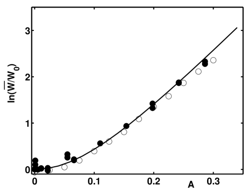
FIG. 3.: The average escape rate $\bar{W}$ for a sinusoidally-driven Duffing oscillator (14) as a function of the field amplitude $A$, $W_{0}$ is the escape rate for $A=0$. The driving frequency is $\omega_{F}=1.2$, the white-noise intensity is $D=0.03$. Solid line: the theoretical expression (13); filled and empty circles are the data from analog and digital simulations, respectively, with no adjustable parameters.

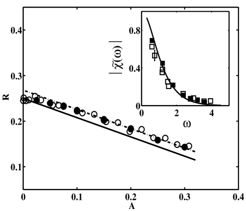
FIG. 4.: The dependence of the activation energy $R$ on the amplitude $A$ of the sinusoidal driving force with $\omega_{F}=1.2$ for the Duffing oscillator as determined by electronic (open circles) and numerical (filled circles) simulations and Eq. (13) (solid line) [25]. The data of analog and digital simulations refer to the noise intensities $0.028<D<0.036$ and $0.020<D<0.028$, respectively. The inset shows the absolute value of the LS of the system $|\tilde{\chi}(\omega)|$ measured (open and filled squares for analog and numerical simulations, respectively) and calculated from (15) [full curve] as a function of frequency $\omega$.

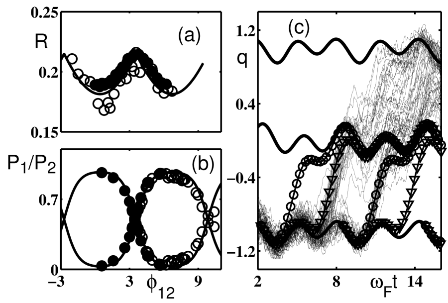
FIG. 5.: (a) The activation energy $R$ as a function of phase difference $\phi_{12}$ with $\omega_{F}=1.2$ for the Duffing oscillator driven by the biharmonic force $F(t)=0.1\cos(\omega_{F}t)+0.3\cos(2\omega_{F}t+\phi_{12})$. Calculations based on (10) (full curve) are compared with data from electronic (open circles) and numerical (filled circles) simulations. (b) Relative numbers of escape trajectories following each escape path in the electronic (filled circles) and numerical (open circles) experiments compared to the calculated relative probabilities (full curve). (c) Measured escape trajectories for the electronic model (thin jagged lines) with the critical phase difference $\phi_{12}=\phi_{cr}\approx 3.57$, compared to the calculated optimal paths (circles and triangles); solid lines are periodic states of (1), (8) in the absence of noise. The data was obtained with the noise intensity $D=0.028$.

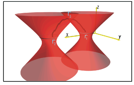
FIG. 6.: Rendering of two focused laser beams, the equilibrium positions of the particle (rings), and a transitional path between the beams

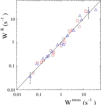
FIG. 7.: Comparison of the measured transition rates $W^{\rm meas}$ and the rates calculated from the three-dimensional Kramers theory, $W^{K}$, using the measured curvatures of the potential wells. The squares represent escapes from the well at ${\bf r}_{1}$ and the triangles represent escapes from the well at ${\bf r}_{2}$ in Fig. 6. The line of slope one indicates the result expected if the three-dimensional Kramers theory correctly predicted the measured transition rates [33].

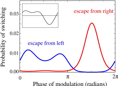
FIG. 8.: The least-squares fits to the experimentally determined instantaneous time-dependent switching probabilities for a particle in the adiabatically modulated double-beam trap, over a cycle $\omega_{F}t$ of the modulating waveform. The phase angle between the first and second harmonics is $\phi_{12}=\pi/2$. When the phase angle was incremented by $\pi$, the escape rates from the left and right wells interchanged, within experimental error. Inset shows the instantaneous difference between the heights of the potential barriers in the two wells.

REFERENCES

- [1] To whom correspondence should be addressed, dykman@pa.msu.edu
- [2] M.I. Dykman, D.G. Luchinsky, R. Mannella, P.V.E. McClintock, N.D. Stein and N.G. Stocks Nuovo Cimento D 17, 661 (1995); L. Gammaitoni, P. Hänggi, P. Jung, and F. Marchesoni, Rev. Mod. Phys. 70, 223 (1998).
- [3] A.I. Larkin and Yu.N. Ovchinnikov, J. Low Temp. Phys. 63, 317 (1986); B.I. Ivlev and V.I. Mel’nikov, Phys. Lett. A 116, 427 (1986); S. Linkwitz and H. Grabert, Phys. Rev. B 44 11888, 11901 (1991); R. Mannella and P. Grigolini, Phys. Rev. B 39, 4722 (1989).
- [4] M.H. Devoret, D. Esteve, J.M. Martinis, A. Cleland, and J. Clarke, Phys. Rev. B 36, 58 (1987); E. Turlot, S. Linkwitz, D. Esteve, C. Urbina, M.H. Devoret, and H. Grabert, Chem. Phys. 235, 47 (1998).
- [5] R. Landauer, J. Stat. Phys. 13, 1 (1975); Phys. Lett. A 68, 15 (1978); J. Stat. Phys. 53, 233 (1988).
- [6] R.S. Maier and D.L. Stein, SIAM J. Appl. Math. 57, 752 (1997).
- [7] P. Jung, Phys. Rep. 234 175 (1993).
- [8] L. E. Reichl and S. Kim, Phys. Rev. E 53, 3088 (1996).
- [9] M. I. Dykman, H. Rabitz, V. N. Smelyanskiy, and B. E. Vugmeister, Phys. Rev. Lett. 79, 1178 (1997).
- [10] V. N. Smelyanskiy, M. I. Dykman, H. Rabitz, and B. E. Vugmeister, Phys. Rev. Lett. 79, 3113 (1997).
- [11] V.N. Smelyanskiy, M.I. Dykman, and B. Golding, Phys. Rev. Lett. 82, 3193–3196 (1999).
- [12] L. Onsager and S. Machlup, Phys. Rev. 91, 1505 (1953).
- [13] M. I. Freidlin and A. D. Wentzel, Random Perturbations in Dynamical Systems (Springer, New-York, 1984).
- [14] M. I. Dykman and M.A. Krivoglaz, Sov. Phys. JETP 50, 30 (1979); in Soviet Physics Reviews, edited by I.M. Khalatnikov (Harwood Academic Publishers, New York, 1984), Vol. 5, pp. 265–442.
- [15] R. Graham and T. Tél, Phys. Rev. Lett. 52, 9 (1984); R. Graham and T. Tél, Phys. Rev. A 31, 1109 (1985); R. Graham, in Noise in Nonlinear Dynamical Systems, edited by F. Moss and P. V. E. McClintock (Cambridge University Press, Cambridge, 1989), Vol. 1, pp. 225–278.
- [16] J.F. Luciani and A.D. Verga, Europhys. Lett. 4, 255 (1987).
- [17] A. Förster and A.S. Mikhailov, Phys. Lett. A 126, 459 (1988).
- [18] A. J. Bray and A. J. McKane, Phys. Rev. Lett. 62, 493 (1989); A.J. McKane, Phys. Rev. A 40, 4050–4053 (1989).
- [19] M.I. Dykman Phys. Rev. A 42, 2020 (1990).
- [20] M.S. Maier and D.L. Stein, J. Stat. Phys. 83, 291 (1996).
- [21] M.I. Dykman and B. Golding, in Stochastic Processes in Physics, Chemistry, and Biology, LNP 557, eds. J.A. Freund and T. Pöschel (Springer-Verlag, Berlin 2000), pp. 246 - 258.
- [22] A different situation occurs if periodic driving is so strong that it makes a metastable state dynamically unstable. An interesting effect of noise in this case was analyzed by I. Dayan, M. Gitterman, and G. H. Weiss, Phys. Rev. A 46, 757 (1992); see also J.M. Casado and M. Morillo, Phys. Rev. E 49, 1136 (1994) and R. N. Mantegna and B. Spagnolo, Phys. Rev. Lett. 76, 563 (1996).
- [23] R.P. Feynman and A.R. Hibbs, Quantum Mechanics and Path Integrals (Mc-Graw Hill, New York 1965).
- [24] M.I. Dykman, M.M. Millonas, and V.N. Smelyanskiy, Phys. Lett. A 195, 53 (1994); M.I. Dykman D.G. Luchinsky, R. Mannella, P.V.E. McClintock, and V.N. Smelyanskiy, Phys. Rev. Lett. 77, 5229 (1996).
- [25] D.G. Luchinsky, R. Mannella, P.V.E. McClintock, M.I. Dykman, and V.N. Smelyanskiy, J. Phys. A 32, L321 (1999).
- [26] H. Kramers, Physica (Utrecht) 7, 284 (1940)
- [27] V.N. Smelyanskiy, M.I. Dykman, H. Rabitz, B.E. Vugmeister, S.L. Bernasek, and A.B. Bocarsly, J. Chem. Phys. 110, 11488 (1999).
- [28] (a) J. Lehman, P. Riemann, and P. Hänggi, Phys. Rev. Lett. 84, 1639 (2000); (b) J. Lehman, P. Riemann, and P. Hänggi, Phys. Rev. E 62, 6282 (2000).
- [29] D.G. Luchinsky, P.V.E. McClintock, and M.I. Dykman, Rep. Prog. Phys. 61, 889 (1998).
- [30] R. Mannella, in Supercomputation in Nonlinear and Disordered Systems, eds. L.Vázquez, F. Tirando, and I. Martin (World Scientific, Singapore, 1997), pp. 100-130.
- [31] A. Ashkin, J. M. Dziedzic, J.E. Bjorkholm, S. Chu, Optics Lett. 11, 288–291 (1986)
- [32] A. Simon and A. Libchaber, Phys. Rev. Lett. 68, 3375–3378 (1992).
- [33] L.I. McCann, M.I. Dykman, and B. Golding, Nature 402, 785–787 (1999).
- [34] M.O. Magnasco, Phys. Rev. Lett. 71, 1477 (1993).
- [35] A. Ajdari, D. Mukamel, L. Paliti, J. Prost, J. Phys. I (France) 4, 1551 (1994); M.C. Mahato and A.M. Jayannavar, Phys. Lett. A 209, 21 (1994); D.R. Chialvo and M.M. Millonas, Phys. Lett. A 209, 26 (1995).
- [36] L.I. McCann and B. Golding, unpublished.
- [37] V.N. Smelyanskiy, in preparation.