A Random Matrix Approach to Cross-Correlations in Financial Data

Abstract

We analyze cross-correlations between price fluctuations of different stocks using methods of random matrix theory (RMT). Using two large databases, we calculate cross-correlation matrices C of returns constructed from (i) 30-min returns of 1000 US stocks for the 2-yr period 1994–95 (ii) 30-min returns of 881 US stocks for the 2-yr period 1996–97, and (iii) 1-day returns of 422 US stocks for the 35-yr period 1962–96. We test the statistics of the eigenvalues $\lambda_{i}$ of C against a “null hypothesis” — a random correlation matrix constructed from mutually uncorrelated time series. We find that a majority of the eigenvalues of C fall within the RMT bounds $[\lambda_{-},\lambda_{+}]$ for the eigenvalues of random correlation matrices. We test the eigenvalues of C within the RMT bound for universal properties of random matrices and find good agreement with the results for the Gaussian orthogonal ensemble of random matrices — implying a large degree of randomness in the measured cross-correlation coefficients. Further, we find that the distribution of eigenvector components for the eigenvectors corresponding to the eigenvalues outside the RMT bound display systematic deviations from the RMT prediction. In addition, we find that these “deviating eigenvectors” are stable in time. We analyze the components of the deviating eigenvectors and find that the largest eigenvalue corresponds to an influence common to all stocks. Our analysis of the remaining deviating eigenvectors shows distinct groups, whose identities correspond to conventionally-identified business sectors. Finally, we discuss applications to the construction of portfolios of stocks that have a stable ratio of risk to return.

PACS numbers: 05.45.Tp, 89.90.+n, 05.40.-a, 05.40.Fb

I Introduction

A Motivation

Quantifying correlations between different stocks is a topic of interest not only for scientific reasons of understanding the economy as a complex dynamical system, but also for practical reasons such as asset allocation and portfolio-risk estimation [2, 3, 1, 4]. Unlike most physical systems, where one relates correlations between subunits to basic interactions, the underlying “interactions” for the stock market problem are not known. Here, we analyze cross-correlations between stocks by applying concepts and methods of random matrix theory, developed in the context of complex quantum systems where the precise nature of the interactions between subunits are not known.

In order to quantify correlations, we first calculate the price change (“return”) of stock $i=1,\dots,N$ over a time scale $\Delta t$

$$G_{i}(t)\equiv\ln S_{i}(t+\Delta t)-\ln S_{i}(t)\,,$$ (1)

where $S_{i}(t)$ denotes the price of stock $i$. Since different stocks have varying levels of volatility (standard deviation), we define a normalized return

$$g_{i}(t)\equiv{G_{i}(t)-\langle G_{i}\rangle\over\sigma_{i}}\,,$$ (2)

where $\sigma_{i}\equiv\sqrt{\langle G_{i}^{2}\rangle-\langle G_{i}\rangle^{2}}$ is the standard deviation of $G_{i}$, and $\langle\cdots\rangle$ denotes a time average over the period studied. We then compute the equal-time cross-correlation matrix C with elements

$$C_{ij}\equiv\langle g_{i}(t)g_{j}(t)\rangle\,.$$ (3)

By construction, the elements $C_{ij}$ are restricted to the domain $-1\leq C_{ij}\leq 1$, where $C_{ij}=1$ corresponds to perfect correlations, $C_{ij}=-1$ corresponds to perfect anti-correlations, and $C_{ij}=0$ corresponds to uncorrelated pairs of stocks.

The difficulties in analyzing the significance and meaning of the empirical cross-correlation coefficients $C_{ij}$ are due to several reasons, which include the following:

(i) Market conditions change with time and the cross-correlations that exist between any pair of stocks may not be stationary.

(ii) The finite length of time series available to estimate cross-correlations introduces “measurement noise”.

If we use a long time series to circumvent the problem of finite length, our estimates will be affected by the non-stationarity of cross-correlations. For these reasons, the empirically-measured cross-correlations will contain “random” contributions, and it is a difficult problem in general to estimate from C the cross-correlations that are not a result of randomness.

How can we identify from $C_{ij}$, those stocks that remained correlated (on the average) in the time period studied? To answer this question, we test the statistics of C against the “null hypothesis” of a random correlation matrix — a correlation matrix constructed from mutually uncorrelated time series. If the properties of C conform to those of a random correlation matrix, then it follows that the contents of the empirically-measured C are random. Conversely, deviations of the properties of C from those of a random correlation matrix convey information about “genuine” correlations. Thus, our goal shall be to compare the properties of C with those of a random correlation matrix and separate the content of C into two groups: (a) the part of C that conforms to the properties of random correlation matrices (“noise”) and (b) the part of C that deviates (“information”).

B Background

The study of statistical properties of matrices with independent random elements — random matrices — has a rich history originating in nuclear physics [5, 6, 7, 8, 9, 10, 11, 12, 13]. In nuclear physics, the problem of interest 50 years ago was to understand the energy levels of complex nuclei, which the existing models failed to explain. RMT was developed in this context by Wigner, Dyson, Mehta, and others in order to explain the statistics of energy levels of complex quantum systems. They postulated that the Hamiltonian describing a heavy nucleus can be described by a matrix H with independent random elements $H_{ij}$ drawn from a probability distribution [5, 6, 7, 8, 9]. Based on this assumption, a series of remarkable predictions were made which are found to be in agreement with the experimental data [5, 6, 7]. For complex quantum systems, RMT predictions represent an average over all possible interactions [8, 9, 10]. Deviations from the universal predictions of RMT identify system-specific, non-random properties of the system under consideration, providing clues about the underlying interactions [11, 12, 13].

Recent studies [14, 15] applying RMT methods to analyze the properties of C show that $\approx 98$% of the eigenvalues of C agree with RMT predictions, suggesting a considerable degree of randomness in the measured cross-correlations. It is also found that there are deviations from RMT predictions for $\approx 2$% of the largest eigenvalues. These results prompt the following questions:

• What is a possible interpretation for the deviations from RMT?

• Are the deviations from RMT stable in time?

• What can we infer about the structure of C from these results?

• What are the practical implications of these results?

In the following, we address these questions in detail. We find that the largest eigenvalue of C represents the influence of the entire market that is common to all stocks. Our analysis of the contents of the remaining eigenvalues that deviate from RMT shows the existence of cross-correlations between stocks of the same type of industry, stocks having large market capitalization, and stocks of firms having business in certain geographical areas [16, 17]. By calculating the scalar product of the eigenvectors from one time period to the next, we find that the “deviating eigenvectors” have varying degrees of time stability, quantified by the magnitude of the scalar product. The largest 2-3 eigenvectors are stable for extended periods of time, while for the rest of the deviating eigenvectors, the time stability decreases as the the corresponding eigenvalues are closer to the RMT upper bound.

To test that the deviating eigenvalues are the only “genuine” information contained in C, we compare the eigenvalue statistics of C with the known universal properties of real symmetric random matrices, and we find good agreement with the RMT results. Using the notion of the inverse participation ratio, we analyze the eigenvectors of C and find large values of inverse participation ratio at both edges of the eigenvalue spectrum — suggesting a “random band” matrix structure for C. Lastly, we discuss applications to the practical goal of finding an investment that provides a given return without exposure to unnecessary risk. In addition, it is possible that our methods can also be applied for filtering out ‘noise’ in empirically-measured cross-correlation matrices in a wide variety of applications.

This paper is organized as follows. Section II contains a brief description of the data analyzed. Section III discusses the statistics of cross-correlation coefficients. Section IV discusses the eigenvalue distribution of C and compares with RMT results. Section V tests the eigenvalue statistics C for universal properties of real symmetric random matrices and Section VI contains a detailed analysis of the contents of eigenvectors that deviate from RMT. Section VII discusses the time stability of the deviating eigenvectors. Section VIII contains applications of RMT methods to construct ‘optimal’ portfolios that have a stable ratio of risk to return. Finally, Section IX contains some concluding remarks.

II Data Analyzed

We analyze two different databases covering securities from the three major US stock exchanges, namely the New York Stock Exchange (NYSE), the American Stock Exchange (AMEX), and the National Association of Securities Dealers Automated Quotation (Nasdaq).

$\bullet$ Database I: We analyze the Trades and Quotes database, that documents all transactions for all major securities listed in all the three stock exchanges. We extract from this database time series of prices [18] of the 1000 largest stocks by market capitalization on the starting date January 3, 1994. We analyze this database for the 2-yr period 1994–95 [19]. From this database, we form $L=6448$ records of 30-min returns of $N=1000$ US stocks for the 2-yr period 1994–95. We also analyze the prices of a subset comprising 881 stocks (of those 1000 we analyze for 1994–95) that survived through two additional years 1996–97. From this data, we extract $L=6448$ records of 30-min returns of $N=881$ US stocks for the 2-yr period 1996–97.

$\bullet$ Database II: We analyze the Center for Research in Security Prices (CRSP) database. The CRSP stock files cover common stocks listed on NYSE beginning in 1925, the AMEX beginning in 1962, and the Nasdaq beginning in 1972. The files provide complete historical descriptive information and market data including comprehensive distribution information, high, low and closing prices, trading volumes, shares outstanding, and total returns. We analyze daily returns for the stocks that survive for the 35-yr period 1962–96 and extract $L=8685$ records of 1-day returns for $N=422$ stocks.

III Statistics of correlation coefficients

We analyze the distribution $P(C_{ij})$ of the elements $\{C_{ij};\,i\neq j\}$ of the cross-correlation matrix C . We first examine $P(C_{ij})$ for 30-min returns from the TAQ database for the 2-yr periods 1994–95 and 1996–97 [Fig. 1(a)]. First, we note that $P(C_{ij})$ is asymmetric and centered around a positive mean value ($\langle C_{ij}\rangle>0$), implying that positively-correlated behavior is more prevalent than negatively-correlated (anti-correlated) behavior. Secondly, we find that $\langle C_{ij}\rangle$ depends on time, e.g., the period 1996–97 shows a larger $\langle C_{ij}\rangle$ than the period 1994–95. We contrast $P(C_{ij})$ with a control — a correlation matrix R with elements $R_{ij}$ constructed from $N=1000$ mutually-uncorrelated time series, each of length $L=6448$, generated using the empirically-found distribution of stock returns [20, 21]. Figure 1(a) shows that $P(R_{ij})$ is consistent with a Gaussian with zero mean, in contrast to $P(C_{ij})$. In addition, we see that the part of $P(C_{ij})$ for $C_{ij}<0$ (which corresponds to anti-correlations) is within the Gaussian curve for the control, suggesting the possibility that the observed negative cross-correlations in C may be an effect of randomness.

Figure 1(b) shows $P(C_{ij})$ for daily returns from the CRSP database for five non-overlapping 7-yr sub-periods in the 35-yr period 1962–96. We see that the time dependence of $\langle C_{ij}\rangle$ is more pronounced in this plot. In particular, the period containing the market crash of October 19, 1987 has the largest average value $\langle C_{ij}\rangle$, suggesting the existence of cross-correlations that are more pronounced in volatile periods than in calm periods. We test this possibility by comparing $\langle C_{ij}\rangle$ with the average volatility of the market (measured using the S&P 500 index), which shows large values of $\langle C_{ij}\rangle$ during periods of large volatility [Fig. 2].

IV Eigenvalue distribution of the correlation matrix

As stated above, our aim is to extract information about cross-correlations from C. So, we compare the properties of C with those of a random cross-correlation matrix [14]. In matrix notation, the correlation matrix can be expressed as

$${\bf\sf C={\rm\it 1\over L}\,G\,G^{T}}\,,$$ (4)

where G is an $N\times L$ matrix with elements $\{g_{i\,m}\equiv g_{i}(m\Delta t)\,;i=1,\dots,N\,;m=0,\dots,L-1\}\,$, and G^T denotes the transpose of G. Therefore, we consider a “random” correlation matrix

$${\bf\sf R={\rm\it 1\over L}\,A\,A^{T}}\,,$$ (5)

where A is an $N\times L$ matrix containing $N$ time series of $L$ random elements with zero mean and unit variance, that are mutually uncorrelated. By construction R belongs to the type of matrices often referred to as Wishart matrices in multivariate statistics [22].

Statistical properties of random matrices such as R are known [23, 24]. Particularly, in the limit $N\rightarrow\infty\,,L\rightarrow\infty$, such that $Q\equiv L/N$ is fixed, it was shown analytically [24] that the distribution $P_{\rm rm}(\lambda)$ of eigenvalues $\lambda$ of the random correlation matrix R is given by

$$P_{\rm rm}(\lambda)={Q\over 2\pi}\,{\sqrt{(\lambda_{+}-\lambda)(\lambda-\lambda_{-})}\over\lambda}\,\,\,,$$ (6)

for $\lambda$ within the bounds $\lambda_{-}\leq\lambda_{i}\leq\lambda_{+}$, where $\lambda_{-}$ and $\lambda_{+}$ are the minimum and maximum eigenvalues of R respectively, given by

$$\lambda_{\pm}=1+{1\over Q}\pm 2\,\sqrt{{1\over Q}}\,.$$ (7)

For finite $L$ and $N$, the abrupt cut-off of $P_{\rm rm}(\lambda)$ is replaced by a rapidly-decaying edge [25].

We next compare the eigenvalue distribution $P(\lambda)$ of C with $P_{\rm rm}(\lambda)$ [14]. We examine $\Delta t=30$ min returns for $N=1000$ stocks, each containing $L=6448$ records. Thus $Q=6.448$, and we obtain $\lambda_{-}=0.36$ and $\lambda_{+}=1.94$ from Eq. (7). We compute the eigenvalues $\lambda_{i}$ of C, where $\lambda_{i}$ are rank ordered ($\lambda_{i+1}>\lambda_{i}$). Figure 3(a) compares the probability distribution $P(\lambda)$ with $P_{\rm rm}(\lambda)$ calculated for $Q=6.448$. We note the presence of a well-defined “bulk” of eigenvalues which fall within the bounds $[\lambda_{-},\lambda_{+}]$ for $P_{\rm rm}(\lambda)$. We also note deviations for a few ($\approx 20$) largest and smallest eigenvalues. In particular, the largest eigenvalue $\lambda_{1000}\approx 50$ for the 2-yr period, which is $\approx 25$ times larger than $\lambda_{+}=1.94$.

Since Eq. (6) is strictly valid only for $L\rightarrow\infty$ and $N\rightarrow\infty$, we must test that the deviations that we find in Fig. 3(a) for the largest few eigenvalues are not an effect of finite values of $L$ and $N$. To this end, we contrast $P(\lambda)$ with the RMT result $P_{\rm rm}(\lambda)$ for the random correlation matrix of Eq. (5), constructed from $N=1000$ separate uncorrelated time series, each of the same length $L=6448$. We find good agreement with Eq. (6) [Fig. 3(b)], thus showing that the deviations from RMT found for the largest few eigenvalues in Fig. 3(a) are not a result of the fact that $L$ and $N$ are finite.

Figure 4 compares $P(\lambda)$ for C calculated using $L=1737$ daily returns of 422 stocks for the 7-yr period 1990–96. We find a well-defined bulk of eigenvalues that fall within $P_{\rm rm}(\lambda)$, and deviations from $P_{\rm rm}(\lambda)$ for large eigenvalues — similar to what we found for $\Delta t=30$ min [Fig. 3(a)]. Thus, a comparison of $P(\lambda)$ with the RMT result $P_{\rm rm}(\lambda)$ allows us to distinguish the bulk of the eigenvalue spectrum of C that agrees with RMT (random correlations) from the deviations (genuine correlations).

V Universal properties: Are the bulk of eigenvalues of C consistent with RMT?

The presence of a well-defined bulk of eigenvalues that agree with $P_{\rm rm}(\lambda)$ suggests that the contents of C are mostly random except for the eigenvalues that deviate. Our conclusion was based on the comparison of the eigenvalue distribution $P(\lambda)$ of C with that of random matrices of the type R = ${1\over L}$ A A^T. Quite generally, comparison of the eigenvalue distribution with $P_{\rm rm}(\lambda)$ alone is not sufficient to support the possibility that the bulk of the eigenvalue spectrum of C is random. Random matrices that have drastically different $P(\lambda)$ share similar correlation structures in their eigenvalues — universal properties — that depend only on the general symmetries of the matrix [11, 12, 13]. Conversely, matrices that have the same eigenvalue distribution can have drastically different eigenvalue correlations. Therefore, a test of randomness of C involves the investigation of correlations in the eigenvalues $\lambda_{i}$.

Since by definition C is a real symmetric matrix, we shall test the eigenvalue statistics C for universal features of eigenvalue correlations displayed by real symmetric random matrices. Consider a $M\times M$ real symmetric random matrix S with off-diagonal elements $S_{ij}$, which for $i<j$ are independent and identically distributed with zero mean $\langle S_{ij}\rangle=0$ and variance $\langle S^{2}_{ij}\rangle>0$. It is conjectured based on analytical [26] and extensive numerical evidence [11] that in the limit $M\rightarrow\infty$, regardless of the distribution of elements $S_{ij}$, this class of matrices, on the scale of local mean eigenvalue spacing, display the universal properties (eigenvalue correlation functions) of the ensemble of matrices whose elements are distributed according to a Gaussian probability measure — called the Gaussian orthogonal ensemble (GOE) [11].

Formally, GOE is defined on the space of real symmetric matrices by two requirements [11]. The first is that the ensemble is invariant under orthogonal transformations, i.e., for any GOE matrix Z, the transformation Z$\rightarrow$Z${}^{\prime}\equiv$W^T Z W, where W is any real orthogonal matrix (W W^T=I), leaves the joint probability $P(Z)dZ$ of elements $Z_{ij}$ unchanged: $P(Z^{\prime})dZ^{\prime}=P(Z)dZ$. The second requirement is that the elements $\{Z_{ij};i\leq j\}$ are statistically independent [11].

By definition, random cross-correlation matrices R (Eq. (5)) that we are interested in are not strictly GOE-type matrices, but rather belong to a special ensemble called the “chiral” GOE [13, 27]. This can be seen by the following argument. Define a matrix B

$$\rm{\bf\sf B}\equiv\left[\begin{array}[]{cc}0&{\bf\sf G}\\ {\bf\sf G}^{T}&0\end{array}\right]\,.$$ (10)

The eigenvalues $\gamma$ of B are given by $\det(\gamma^{2}{\bf\sf I}-{\bf\sf GG}^{T})=0$ and similarly, the eigenvalues $\lambda$ of R are given by $\det(\lambda{\bf\sf I}-{\bf\sf GG}^{T})=0$. Thus, all non-zero eigenvalues of B occur in pairs, i.e., for every eigenvalue $\lambda$ of R, $\gamma_{\pm}=\pm\sqrt{\lambda}$ are eigenvalues of B. Since the eigenvalues occur pairwise, the eigenvalue spectra of both B and R have special properties in the neighborhood of zero that are different from the standard GOE [13, 27]. As these special properties decay rapidly as one goes further from zero, the eigenvalue correlations of R in the bulk of the spectrum are still consistent with those of the standard GOE. Therefore, our goal shall be to test the bulk of the eigenvalue spectrum of the empirically-measured cross-correlation matrix C with the known universal features of standard GOE-type matrices.

In the following, we test the statistical properties of the eigenvalues of C for three known universal properties [11, 12, 13] displayed by GOE matrices: (i) the distribution of nearest-neighbor eigenvalue spacings $P_{\rm nn}(s)$, (ii) the distribution of next-nearest-neighbor eigenvalue spacings $P_{\rm nnn}(s)$, and (iii) the “number variance” statistic $\Sigma^{2}$.

The analytical results for the three properties listed above hold if the spacings between adjacent eigenvalues (rank-ordered) are expressed in units of average eigenvalue spacing. Quite generally, the average eigenvalue spacing changes from one part of the eigenvalue spectrum to the next. So, in order to ensure that the eigenvalue spacing has a uniform average value throughout the spectrum, we must find a transformation called “unfolding,” which maps the eigenvalues $\lambda_{i}$ to new variables called “unfolded eigenvalues” $\xi_{i}$, whose distribution is uniform [11, 12, 13]. Unfolding ensures that the distances between eigenvalues are expressed in units of local mean eigenvalue spacing [11], and thus facilitates comparison with theoretical results. The procedures that we use for unfolding the eigenvalue spectrum are discussed in Appendix A.

A Distribution of nearest-neighbor eigenvalue spacings

We first consider the eigenvalue spacing distribution, which reflects two-point as well as eigenvalue correlation functions of all orders. We compare the eigenvalue spacing distribution of C with that of GOE random matrices. For GOE matrices, the distribution of “nearest-neighbor” eigenvalue spacings $s\equiv\xi_{k+1}-\xi_{k}$ is given by [11, 12, 13]

$$P_{\rm GOE}(s)={\pi s\over 2}\,\exp\left(-{\pi\over 4}\,s^{2}\right)\,,$$ (11)

often referred to as the “Wigner surmise” [28]. The Gaussian decay of $P_{\rm GOE}(s)$ for large $s$ [bold curve in Fig. 5(a)] implies that $P_{\rm GOE}(s)$ “probes” scales only of the order of one eigenvalue spacing. Thus, the spacing distribution is known to be robust across different unfolding procedures [13].

We first calculate the distribution of the “nearest-neighbor spacings” $s\equiv\xi_{k+1}-\xi_{k}$ of the unfolded eigenvalues obtained using the Gaussian broadening procedure. Figure 5(a) shows that the distribution $P_{\rm nn}(s)$ of nearest-neighbor eigenvalue spacings for C constructed from 30-min returns for the 2-yr period 1994–95 agrees well with the RMT result $P_{\rm GOE}(s)$ for GOE matrices.

Identical results are obtained when we use the alternative unfolding procedure of fitting the eigenvalue distribution. In addition, we test the agreement of $P_{\rm nn}(s)$ with RMT results by fitting $P_{\rm nn}(s)$ to the one-parameter Brody distribution [12, 13]

$$P_{\rm Br}(s)=B\,(1+\beta)\,s^{\beta}\,\exp(-Bs^{1+\beta})\,,$$ (12)

where $B\equiv[\Gamma({\beta+2\over\beta+1})]^{1+\beta}$. The case $\beta=1$ corresponds to the GOE and $\beta=0$ corresponds to uncorrelated eigenvalues (Poisson-distributed spacings). We obtain $\beta=0.99\pm 0.02$, in good agreement with the GOE prediction $\beta=1$. To test non-parametrically that $P_{\rm GOE}(s)$ is the correct description for $P_{\rm nn}(s)$, we perform the Kolmogorov-Smirnov test. We find that at the 60$\%$ confidence level, a Kolmogorov-Smirnov test cannot reject the hypothesis that the GOE is the correct description for $P_{\rm nn}(s)$.

Next, we analyze the nearest-neighbor spacing distribution $P_{\rm nn}(s)$ for C constructed from daily returns for four 7-yr periods [Fig. 6]. We find good agreement with the GOE result of Eq. (11), similar to what we find for C constructed from 30-min returns. We also test that both of the unfolding procedures discussed in Appendix A yield consistent results. Thus, we have seen that the eigenvalue-spacing distribution of empirically-measured cross-correlation matrices C is consistent with the RMT result for real symmetric random matrices.

B Distribution of next-nearest-neighbor eigenvalue spacings

A second independent test for GOE is the distribution $P_{\rm nnn}(s^{\prime})$ of next-nearest-neighbor spacings $s^{\prime}\equiv\xi_{k+2}-\xi_{k}$ between the unfolded eigenvalues. For matrices of the GOE type, according to a theorem due to Ref. [10], the next-nearest neighbor spacings follow the statistics of the Gaussian symplectic ensemble (GSE) [11, 12, 13, 29]. In particular, the distribution of next-nearest-neighbor spacings $P_{\rm nnn}(s^{\prime})$ for a GOE matrix is identical to the distribution of nearest-neighbor spacings of the Gaussian symplectic ensemble (GSE) [11, 13]. Figure 5(b) shows that $P_{\rm nnn}(s^{\prime})$ for the same data as Fig. 5(a) agrees well with the RMT result for the distribution of nearest-neighbor spacings of GSE matrices,

$$P_{\rm GSE}(s)={2^{18}\over 3^{6}\pi^{3}}\,s^{4}\,\exp\left(-{64\over 9\pi}\,s^{2}\right)\,.$$ (13)

C Long-range eigenvalue correlations

To probe for larger scales, pair correlations (“two-point” correlations) in the eigenvalues, we use the statistic $\Sigma^{2}$ often called the “number variance,” which is defined as the variance of the number of unfolded eigenvalues in intervals of length $\ell$ around each $\xi_{i}$ [11, 12, 13],

$$\Sigma^{2}(\ell)\equiv\langle[n(\xi,\ell)-\ell]^{2}\rangle_{\xi}\,,$$ (14)

where $n(\xi,\ell)$ is the number of unfolded eigenvalues in the interval $[\xi-\ell/2,\xi+\ell/2]$ and $\langle\dots\rangle_{\xi}$ denotes an average over all $\xi$. If the eigenvalues are uncorrelated, $\Sigma^{2}\sim\ell$. For the opposite extreme of a “rigid” eigenvalue spectrum (e.g. simple harmonic oscillator), $\Sigma^{2}$ is a constant. Quite generally, the number variance $\Sigma^{2}$ can be expressed as

$$\Sigma^{2}(\ell)=\ell-2\,\int_{0}^{\ell}\,(\ell-x)\,Y(x)dx\,,$$ (15)

where $Y(x)$ (called “two-level cluster function”) is related to the two-point correlation function [c.f., Ref. [11], pp.79]. For the GOE case, $Y(x)$ is explicitly given by

$$Y(x)\equiv s^{2}(x)+{ds\over dx}\,\int_{x}^{\infty}s(x^{\prime})dx^{\prime}\,,$$ (16)

where

$$s(x)\equiv{\sin(\pi x)\over\pi x}\,.$$ (17)

For large values of $\ell$, the number variance $\Sigma^{2}$ for GOE has the “intermediate” behavior

$$\Sigma^{2}\sim\ln\ell.$$ (18)

Figure 7 shows that $\Sigma^{2}(\ell)$ for C calculated using 30-min returns for 1994–95 agrees well with the RMT result of Eq. (15). For the range of $\ell$ shown in Fig. 7, both unfolding procedures yield similar results. Consistent results are obtained for C constructed from daily returns.

D Implications

To summarize this section, we have tested the statistics of C for universal features of eigenvalue correlations displayed by GOE matrices. We have seen that the distribution of the nearest-neighbor spacings $P_{\rm nn}(s)$ is in good agreement with the GOE result. To test whether the eigenvalues of C display the RMT results for long-range two-point eigenvalue correlations, we analyzed the number variance $\Sigma^{2}$ and found good agreement with GOE results. Moreover, we also find that the statistics of next-nearest neighbor spacings conform to the predictions of RMT. These findings show that the statistics of the bulk of the eigenvalues of the empirical cross-correlation matrix C is consistent with those of a real symmetric random matrix. Thus, information about genuine correlations are contained in the deviations from RMT, which we analyze below.

VI Statistics of eigenvectors

A Distribution of eigenvector components

The deviations of $P(\lambda)$ from the RMT result $P_{\rm rm}(\lambda)$ suggests that these deviations should also be displayed in the statistics of the corresponding eigenvector components [14]. Accordingly, in this section, we analyze the distribution of eigenvector components. The distribution of the components $\{u^{k}_{l};l=1,\dots,N\}$ of eigenvector u^k of a random correlation matrix R should conform to a Gaussian distribution with mean zero and unit variance [13],

$$\rho_{\rm rm}(u)={1\over\sqrt{2\pi}}\exp({-u^{2}\over 2})\,.$$ (19)

First, we compare the distribution of eigenvector components of C with Eq. (19). We analyze $\rho(u)$ for C computed using 30-min returns for 1994–95. We choose one typical eigenvalue $\lambda_{k}$ from the bulk ($\lambda_{-}\leq\lambda_{k}\leq\lambda_{+}$) defined by $P_{\rm rm}(\lambda)$ of Eq. (6). Figure 8(a) shows that $\rho(u)$ for a typical u^k from the bulk shows good agreement with the RMT result $\rho_{\rm rm}(u)$. Similar analysis on the other eigenvectors belonging to eigenvalues within the bulk yields consistent results, in agreement with the results of the previous sections that the bulk agrees with random matrix predictions. We test the agreement of the distribution $\rho(u)$ with $\rho_{\rm rm}(u)$ by calculating the kurtosis, which for a Gaussian has the value $3$. We find significant deviations from $\rho_{\rm rm}(u)$ for $\approx 20$ largest and smallest eigenvalues. The remaining eigenvectors have values of kurtosis that are consistent with the Gaussian value $3$.

Consider next the “deviating” eigenvalues $\lambda_{i}$, larger than the RMT upper bound, $\lambda_{i}>\lambda_{+}$. Figure 8(b) and (c) show that, for deviating eigenvalues, the distribution of eigenvector components $\rho(u)$ deviates systematically from the RMT result $\rho_{\rm rm}(u)$. Finally, we examine the distribution of the components of the eigenvector u¹⁰⁰⁰ corresponding to the largest eigenvalue $\lambda_{1000}$. Figure 8(d) shows that $\rho(u^{1000})$ deviates remarkably from a Gaussian, and is approximately uniform, suggesting that all stocks participate. In addition, we find that almost all components of u¹⁰⁰⁰ have the same sign, thus causing $\rho(u)$ to shift to one side. This suggests that the significant participants of eigenvector u^k have a common component that affects all of them with the same bias.

B Interpretation of the largest eigenvalue and the corresponding eigenvector

Since all components participate in the eigenvector corresponding to the largest eigenvalue, it represents an influence that is common to all stocks. Thus, the largest eigenvector quantifies the qualitative notion that certain newsbreaks (e.g., an interest rate increase) affect all stocks alike [4]. One can also interpret the largest eigenvalue and its corresponding eigenvector as the collective ‘response’ of the entire market to stimuli. We quantitatively investigate this notion by comparing the projection (scalar product) of the time series G on the eigenvector u¹⁰⁰⁰, with a standard measure of US stock market performance — the returns $G_{\rm SP}(t)$ of the S&P 500 index. We calculate the projection $G^{1000}(t)$ of the time series $G_{j}(t)$ on the eigenvector u¹⁰⁰⁰,

$$G^{1000}(t)\equiv\sum_{j=1}^{1000}u^{1000}_{j}\,G_{j}(t)\,.$$ (20)

By definition, $G^{1000}(t)$ shows the return of the portfolio defined by u¹⁰⁰⁰. We compare $G^{1000}(t)$ with $G_{\rm SP}(t)$, and find remarkably similar behavior for the two, indicated by a large value of the correlation coefficient $\langle G_{\rm SP}(t)G^{1000}(t)\rangle=0.85$. Figure 9 shows $G^{1000}(t)$ regressed against $G_{SP}(t)$, which shows relatively narrow scatter around a linear fit. Thus, we interpret the eigenvector u¹⁰⁰⁰ as quantifying market-wide influences on all stocks [14, 15].

We analyze C at larger time scales of $\Delta t=1$ day and find similar results as above, suggesting that similar correlation structures exist for quite different time scales. Our results for the distribution of eigenvector components agree with those reported in Ref. [14], where $\Delta t=1$ day returns are analyzed. We next investigate how the largest eigenvalue changes as a function of time. Figure 2 shows the time dependence [30] of the largest eigenvalue ($\lambda_{422}$) for the 35-yr period 1962–96. We find large values of the largest eigenvalue during periods of high market volatility, which suggests strong collective behavior in regimes of high volatility.

One way of statistically modeling an influence that is common to all stocks is to express the return $G_{i}$ of stock $i$ as

$$G_{i}(t)=\alpha_{i}+\beta_{i}M(t)+\epsilon_{i}(t)\,,$$ (21)

where $M(t)$ is an additive term that is the same for all stocks, $\langle\epsilon(t)\rangle=0$, $\alpha_{i}$ and $\beta_{i}$ are stock-specific constants, and $\langle M(t)\epsilon(t)\rangle=0$. This common term $M(t)$ gives rise to correlations between any pair of stocks. The decomposition of Eq. (21) forms the basis of widely-used economic models, such as multi-factor models and the Capital Asset Pricing Model [4, 31, 32, 33, 34, 35, 36, 37, 38, 39, 40, 41, 42, 43, 44, 45, 46, 47]. Since u¹⁰⁰⁰ represents an influence that is common to all stocks, we can approximate the term $M(t)$ with $G^{1000}(t)$. The parameters $\alpha_{i}$ and $\beta_{i}$ can therefore be estimated by an ordinary least squares regression.

Next, we remove the contribution of $G^{1000}(t)$ to each time series $G_{i}(t)$, and construct C from the residuals $\epsilon_{i}(t)$ of Eq. (21). Figure 10 shows that the distribution $P(C_{ij})$ thus obtained has significantly smaller average value $\langle C_{ij}\rangle$, showing that a large degree of cross-correlations contained in C can be attributed to the influence of the largest eigenvalue (and its corresponding eigenvector) [48, 49].

C Number of significant participants in an eigenvector: Inverse Participation Ratio

Having studied the interpretation of the largest eigenvalue which deviates significantly from RMT results, we next focus on the remaining eigenvalues. The deviations of the distribution of components of an eigenvector u^k from the RMT prediction of a Gaussian is more pronounced as the separation from the RMT upper bound $\lambda_{k}-\lambda_{+}$ increases. Since proximity to $\lambda_{+}$ increases the effects of randomness, we quantify the number of components that participate significantly in each eigenvector, which in turn reflects the degree of deviation from RMT result for the distribution of eigenvector components. To this end, we use the notion of the inverse participation ratio (IPR), often applied in localization theory [13, 50]. The IPR of the eigenvector u^k is defined as

$$I^{k}\equiv\sum_{l=1}^{N}\,[u^{k}_{l}]~{}^{4}\,,$$ (22)

where $u^{k}_{l}$, $l=1,\dots,1000$ are the components of eigenvector u^k. The meaning of $I^{k}$ can be illustrated by two limiting cases: (i) a vector with identical components $u^{k}_{l}\equiv 1/\sqrt{N}$ has $I^{k}=1/N$, whereas (ii) a vector with one component $u^{k}_{1}=1$ and the remainder zero has $I^{k}=1$. Thus, the IPR quantifies the reciprocal of the number of eigenvector components that contribute significantly.

Figure 11(a) shows $I^{k}$ for the case of the control of Eq. (5) using time series with the empirically-found distribution of returns [20]. The average value of $I^{k}$ is $\langle I\rangle\approx 3\times 10^{-3}\approx 1/N$ with a narrow spread, indicating that the vectors are extended [50, 51]—i.e., almost all components contribute to them. Fluctuations around this average value are confined to a narrow range (standard deviation of $1.5\times 10^{-4}$).

Figure 11(b) shows that $I^{k}$ for C constructed from 30-min returns from the period 1994–95, agrees with $I^{k}$ of the random control in the bulk ($\lambda_{-}<\lambda_{i}<\lambda_{+}$). In contrast, the edges of the eigenvalue spectrum of C show significant deviations of $I^{k}$ from $\langle I\rangle$. The largest eigenvalue has $1/I^{k}\approx 600$ for the 30-min data [Fig. 11(b)] and $1/I^{k}\approx 320$ for the 1-day data [Fig. 11(c) and (d)], showing that almost all stocks participate in the largest eigenvector. For the rest of the large eigenvalues which deviate from the RMT upper bound, $I^{k}$ values are approximately 4-5 times larger than $\langle I\rangle$, showing that there are varying numbers of stocks contributing to these eigenvectors. In addition, we also find that there are large $I^{k}$ values for vectors corresponding to few of the small eigenvalues $\lambda_{i}\approx 0.25<\lambda_{-}$. The deviations at both edges of the eigenvalue spectrum are considerably larger than $\langle I\rangle$, which suggests that the vectors are localized [50, 51]—i.e., only a few stocks contribute to them.

The presence of vectors with large values of $I^{k}$ also arises in the theory of Anderson localization[52]. In the context of localization theory, one frequently finds “random band matrices”[50] containing extended states with small $I^{k}$ in the bulk of the eigenvalue spectrum, whereas edge states are localized and have large $I^{k}$. Our finding of localized states for small and large eigenvalues of the cross-correlation matrix C is reminiscent of Anderson localization and suggests that C may have a random band matrix structure. A random band matrix B has elements $B_{ij}$ independently drawn from different probability distributions. These distributions are often taken to be Gaussian parameterized by their variance, which depends on $i$ and $j$. Although such matrices are random, they still contain probabilistic information arising from the fact that a metric can be defined on their set of indices $i$. A related, but distinct way of analyzing cross-correlations by defining ‘ultra-metric’ distances has been studied in Ref. [16].

D Interpretation of deviating eigenvectors u⁹⁹⁰–u⁹⁹⁹

We quantify the number of significant participants of an eigenvector using the IPR, and we examine the $1/I^{k}$ components of eigenvector u^k for common features [17]. A direct examination of these eigenvectors, however, does not yield a straightforward interpretation of their economic relevance. To interpret their meaning, we note that the largest eigenvalue is an order of magnitude larger than the others, which constrains the remaining $N-1$ eigenvalues since Tr C $=N$. Thus, in order to analyze the deviating eigenvectors, we must remove the effect of the largest eigenvalue $\lambda_{1000}$.

In order to avoid the effect of $\lambda_{1000}$, and thus $G^{1000}(t)$, on the returns of each stock $G_{i}(t)$, we perform the regression of Eq. (21), and compute the residuals $\epsilon_{i}(t)$. We then calculate the correlation matrix C using $\epsilon_{i}(t)$ in Eq.( 2) and Eq. (3). Next, we compute the eigenvectors u^k of C thus obtained, and analyze their significant participants. The eigenvector u⁹⁹⁹ contains approximately $1/I^{999}=300$ significant participants, which are all stocks with large values of market capitalization. Figure 12 shows that the magnitude of the eigenvector components of u⁹⁹⁹ shows an approximately logarithmic dependence on the market capitalizations of the corresponding stocks.

We next analyze the significant contributors of the rest of the eigenvectors. We find that each of these deviating eigenvectors contains stocks belonging to similar or related industries as significant contributors. Table I shows the ticker symbols and industry groups (Standard Industry Classification (SIC) code) for stocks corresponding to the ten largest eigenvector components of each eigenvector. We find that these eigenvectors partition the set of all stocks into distinct groups which contain stocks with large market capitalization (u⁹⁹⁹), stocks of firms in the electronics and computer industry (u⁹⁹⁸), a combination of gold mining and investment firms (u⁹⁹⁶ and u⁹⁹⁷), banking firms (u⁹⁹⁴), oil and gas refining and equipment (u⁹⁹³), auto manufacturing firms (u⁹⁹²), drug manufacturing firms (u⁹⁹¹), and paper manufacturing (u⁹⁹⁰). One eigenvector (u⁹⁹⁵) displays a mixture of three industry groups — telecommunications, metal mining, and banking. An examination of these firms shows significant business activity in Latin America. Our results are also represented schematically in Fig. 13. A similar classification of stocks into sectors using different methods is obtained in Ref. [16].

Instead of performing the regression of Eq( 21), one can remove the U-shaped intra-daily pattern using the procedure of Ref [53] and compute C. The results thus obtained are consistent with those obtained using the procedure of using the residuals of the regression of Eq. (21) to compute C (Table I). Often C is constructed from returns at longer time scales of $\Delta t=1$ week or 1 month to avoid short time scale effects [54].

E Smallest eigenvalues and their corresponding eigenvectors

Having examined the largest eigenvalues, we next focus on the smallest eigenvalues which show large values of $I^{k}$ [Fig. 11]. We find that the eigenvectors corresponding to the smallest eigenvalues contain as significant participants, pairs of stocks which have the largest values of $C_{ij}$ in our sample. For example, the two largest components of u¹ correspond to the stocks of Texas Instruments (TXN) and Micron Technology (MU) with $C_{ij}=0.64$, the largest correlation coefficient in our sample. The largest components of u² are Telefonos de Mexico (TMX) and Grupo Televisa (TV) with $C_{ij}=0.59$ (second largest correlation coefficient). The eigenvector u³ shows Newmont Gold Company (NGC) and Newmont Mining Corporation (NEM) with $C_{ij}=0.50$ (third largest correlation coefficient) as largest components. In all three eigenvectors, the relative sign of the two largest components is negative. Thus pairs of stocks with a correlation coefficient much larger than the average $\langle C_{ij}\rangle$ effectively “decouple” from other stocks.

The appearance of strongly correlated pairs of stocks in the eigenvectors corresponding to the smallest eigenvalues of C can be qualitatively understood by considering the example of a $2\times 2$ cross-correlation matrix

$$\rm{\bf\sf C}_{2\times 2}=\left[\begin{array}[]{cc}1&c\\ c&1\end{array}\right]\ \ .$$ (25)

The eigenvalues of C_2×2 are $\beta_{\pm}=1\pm c$. The smaller eigenvalue $\beta_{-}$ decreases monotonically with increasing cross-correlation coefficient $c$. The corresponding eigenvector is the anti-symmetric linear combination of the basis vectors $\left(\begin{array}[]{c}1\\ 0\end{array}\right)$ and $\left(\begin{array}[]{c}0\\ 1\end{array}\right)$, in agreement with our empirical finding that the relative sign of largest components of eigenvectors corresponding to the smallest eigenvalues is negative. In this simple example, the symmetric linear combination of the two basis vectors appears as the eigenvector of the large eigenvalue $\beta_{+}$. Indeed, we find that TXN and MU are the largest components of u⁹⁹⁸, TMX and TV are the largest components of u⁹⁹⁵, and NEM and NGC are the largest and third largest components of u⁹⁹⁷.

VII Stability of eigenvectors in time

We next investigate the degree of stability in time of the eigenvectors corresponding to the eigenvalues that deviate from RMT results. Since deviations from RMT results imply genuine correlations which remain stable in the period used to compute C, we expect the deviating eigenvectors to show some degree of time stability.

We first identify the $p$ eigenvectors corresponding to the $p$ largest eigenvalues which deviate from the RMT upper bound $\lambda_{+}$. We then construct a $p\times N$ matrix D with elements $D_{kj}=\{u^{k}_{j}\,;k=1,\dots,p\,;j=1,\dots,N\}$. Next, we compute a $p\times p$ “overlap matrix” O($t,\tau$) = D_A D${}_{B}^{T}$, with elements $O_{ij}$ defined as the scalar product of eigenvector uⁱ of period A (starting at time $t=t$) with u^j of period B at a later time $t+\tau$,

$$O_{ij}(t,\tau)\equiv\sum_{k=1}^{N}D_{ik}(t)D_{jk}(t+\tau)\,.$$ (26)

If all the $p$ eigenvectors are “perfectly” non-random and stable in time $O_{ij}=\delta_{ij}$.

We study the overlap matrices O using both high-frequency and daily data. For high-frequency data ($L=6448$ records at 30-min intervals), we use a moving window of length $L=1612$, and slide it through the entire 2-yr period using discrete time steps $L/4=403$. We first identify the eigenvectors of the correlation matrices for each of these time periods. We then calculate overlap matrices O($t=0,\tau=nL/4$), where $n\in\{1,2,3,\dots\}$, between the eigenvectors for $t=0$ and for $t=\tau$.

Figure 14 shows a grey scale pixel-representation of the matrix O ($t,\tau$), for different $\tau$. First, we note that the eigenvectors that deviate from RMT bounds show varying degrees of stability ($O_{ij}(t,\tau)$) in time. In particular, the stability in time is largest for u¹⁰⁰⁰. Even at lags of $\tau=1$ yr the corresponding overlap $\approx 0.85$. The remaining eigenvectors show decreasing amounts of stability as the RMT upper bound $\lambda_{+}$ is approached. In particular, the 3-4 largest eigenvectors show large values of $O_{ij}$ for up to $\tau=1$ yr.

Next, we repeat our analysis for daily returns of 422 stocks using $8685$ records of 1-day returns, and a sliding window of length $L=965$ with discrete time steps $L/5=193$ days. Instead of calculating O($t,\tau$) for all starting points $t$, we calculate O($\tau$)$\equiv\langle$ O($t,\tau$) $\rangle_{t}$, averaged over all $t=n\,L/5$, where $n\in\{0,1,2,\dots\}$. Figure 15 shows grey scale representations of O ($\tau$) for increasing $\tau$. We find similar results as found for shorter time scales, and find that eigenvectors corresponding to the largest 2 eigenvalues are stable for time scales as large as $\tau=$20 yr. In particular, the eigenvector u⁴²² shows an overlap of $\approx 0.8$ even over time scales of $\tau=$30 yr.

VIII Applications to portfolio optimization

The randomness of the “bulk” seen in the previous sections has implications in optimal portfolio selection [54]. We illustrate these using the Markowitz theory of optimal portfolio selection [3, 55, 17]. Consider a portfolio $\Pi(t)$ of stocks with prices $S_{i}$. The return on $\Pi(t)$ is given by

$$\Phi=\sum_{i=1}^{N}w_{i}G_{i}\,,$$ (27)

where $G_{i}(t)$ is the return on stock $i$ and $w_{i}$ is the fraction of wealth invested in stock $i$. The fractions $w_{i}$ are normalized such that $\sum_{i=1}^{N}w_{i}=1$. The risk in holding the portfolio $\Pi(t)$ can be quantified by the variance

$$\Omega^{2}=\sum_{i=1}^{N}\sum_{j=1}^{N}w_{i}w_{j}C_{ij}\sigma_{i}\sigma_{j}\,,$$ (28)

where $\sigma_{i}$ is the standard deviation (average volatility) of $G_{i}$, and $C_{ij}$ are elements of the cross-correlation matrix C. In order to find an optimal portfolio, we must minimize $\Omega^{2}$ under the constraint that the return on the portfolio is some fixed value $\Phi$. In addition, we also have the constraint that $\sum_{i=1}^{N}w_{i}=1$. Minimizing $\Omega^{2}$ subject to these two constraints can be implemented by using two Lagrange multipliers, which yields a system of linear equations for $w_{i}$, which can then be solved. The optimal portfolios thus chosen can be represented as a plot of the return $\Phi$ as a function of risk $\Omega^{2}$ [Fig. 16].

To find the effect of randomness of C on the selected optimal portfolio, we first partition the time period 1994–95 into two one-year periods. Using the cross-correlation matrix C₉₄ for 1994, and $G_{i}$ for 1995, we construct a family of optimal portfolios, and plot $\Phi$ as a function of the predicted risk $\Omega_{\rm p}^{2}$ for 1995 [Fig. 16(a)]. For this family of portfolios, we also compute the risk $\Omega_{\rm r}^{2}$ realized during 1995 using C₉₅ [Fig. 16(a)]. We find that the predicted risk is significantly smaller when compared to the realized risk,

$${\Omega_{\rm r}^{2}-\Omega_{\rm p}^{2}\over\Omega_{\rm p}^{2}}\approx 170\%\,.$$ (29)

Since the meaningful information in C is contained in the deviating eigenvectors (whose eigenvalues are outside the RMT bounds), we must construct a ‘filtered’ correlation matrix C^′, by retaining only the deviating eigenvectors. To this end, we first construct a diagonal matrix $\Lambda^{\prime}$, with elements $\Lambda^{\prime}_{ii}=\{0,\dots,0,\lambda_{988},\dots,\lambda_{1000}\}$. We then transform $\Lambda^{\prime}$ to the basis of C, thus obtaining the ‘filtered’ cross-correlation matrix C^′. In addition, we set the diagonal elements $C^{\prime}_{ii}=1$, to preserve ${\rm Tr}$(C) $=$ ${\rm Tr}$(C^′) $=N$. We repeat the above calculations for finding the optimal portfolio using C^′ instead of C in Eq. (28). Figure 16(b) shows that the realized risk is now much closer to the predicted risk

$${\Omega_{\rm r}^{2}-\Omega_{\rm p}^{2}\over\Omega_{\rm p}^{2}}\approx 25\%\,.$$ (30)

Thus, the optimal portfolios constructed using C^′ are significantly more stable in time.

IX Conclusions

How can we understand the deviating eigenvalues — i.e., correlations that are stable in time? One approach is to postulate that returns can be separated into idiosyncratic and common components — i.e., that returns can be separated into different additive “factors”, which represent various economic influences that are common to a set of stocks such as the type of industry, or the effect of news [4, 31, 32, 33, 34, 35, 36, 37, 38, 39, 40, 41, 42, 43, 44, 45, 46, 47, 56, 57, 48, 49].

On the other hand, in physical systems one starts from the interactions between the constituents, and then relates interactions to correlated “modes” of the system. In economic systems, we ask if a similar mechanism can give rise to the correlated behavior. In order to answer this question, we model stock price dynamics by a family of stochastic differential equations [59], which describe the ‘instantaneous” returns $g_{i}(t)={d\over dt}\ln S_{i}(t)$ as a random walk with couplings $J_{ij}$

$$\tau_{o}\partial_{t}g_{i}(t)=-r_{i}g_{i}(t)-\kappa g_{i}^{3}(t)+\sum_{j}J_{ij}g_{j}(t)+{1\over\tau_{o}}\xi_{i}(t)\ \ \,.$$ (31)

Here, $\xi_{i}(t)$ are Gaussian random variables with correlation function $\langle\xi_{i}(t)\xi_{j}(t^{\prime})\rangle=\delta_{ij}\tau_{o}\delta(t-t^{\prime})$, and $\tau_{o}$ sets the time scale of the problem. In the context of a soft spin model, the first two terms in the rhs of Eq. (31) arise from the derivative of a double-well potential, enforcing the soft spin constraint. The interaction among soft-spins is given by the couplings $J_{ij}$. In the absence of the cubic term, and without interactions, $\tau_{o}/r_{i}$ are relaxation times of the $\langle g_{i}(t)g_{i}(t+\tau)\rangle$ correlation function. The return $G_{i}$ at a finite time interval $\Delta t$ is given by the integral of $g_{i}$ over $\Delta t$.

Equation (31) is similar to the linearized description of interacting “soft spins” [58] and is a generalized case of the models of Refs. [59]. Without interactions, the variance of price changes on a scale $\Delta t\gg\tau_{i}$ is given by $\langle(G_{i}(\Delta t))^{2}\rangle=\Delta t/(r^{2}\tau_{i})$, in agreement with recent studies [61], where stock price changes are described by an anomalous diffusion and the variance of price changes is decomposed into a product of trading frequency (analog of $1/\tau_{i}$) and the square of an “impact parameter” which is related to liquidity (analog of $1/r$).

As the coupling strengths increase, the soft-spin system undergoes a transition to an ordered state with permanent local magnetizations. At the transition point, the spin dynamics are very “slow” as reflected in a power law decay of the spin autocorrelation function in time. To test whether this signature of strong interactions is present for the stock market problem, we analyze the correlation functions $c^{(k)}(\tau)\equiv\langle G^{(k)}(t)G^{(k)}(t+\tau)\rangle$, where $G^{(k)}(t)\equiv\sum_{i=1}^{1000}u_{i}^{k}G_{i}(t)$ is the time series defined by eigenvector u^k. Instead of analyzing $c^{(k)}(\tau)$ directly, we apply the detrended fluctuation analysis (DFA) method [60]. Figure 17 shows that the correlation functions $c^{(k)}(\tau)$ indeed decay as power laws  [62] for the deviating eigenvectors u^k — in sharp contrast to the behavior of $c^{(k)}(\tau)$ for the rest of the eigenvectors and the autocorrelation functions of individual stocks, which show only short-ranged correlations. We interpret this as evidence for strong interactions [63].

In the absence of the non-linearities (cubic term), we obtain only exponentially-decaying correlation functions for the “modes” corresponding to the large eigenvalues, which is inconsistent with our finding of power-law correlations.

To summarize, we have tested the eigenvalue statistics of the empirically-measured correlation matrix C against the null hypothesis of a random correlation matrix. This allows us to distinguish genuine correlations from “apparent” correlations that are present even for random matrices. We find that the bulk of the eigenvalue spectrum of C shares universal properties with the Gaussian orthogonal ensemble of random matrices. Further, we analyze the deviations from RMT, and find that (i) the largest eigenvalue and its corresponding eigenvector represent the influence of the entire market on all stocks, and (ii) using the rest of the deviating eigenvectors, we can partition the set of all stocks studied into distinct subsets whose identity corresponds to conventionally-identified business sectors. These sectors are stable in time, in some cases for as many as 30 years. Finally, we have seen that the deviating eigenvectors are useful for the construction of optimal portfolios which have a stable ratio of risk to return.

A “Unfolding” the eigenvalue distribution

As discussed in Section V, random matrices display universal functional forms for eigenvalue correlations that depend only on the general symmetries of the matrix. A first step to test the data for such universal properties is to find a transformation called “unfolding,” which maps the eigenvalues $\lambda_{i}$ to new variables called “unfolded eigenvalues” $\xi_{i}$, whose distribution is uniform [11, 12, 13]. Unfolding ensures that the distances between eigenvalues are expressed in units of local mean eigenvalue spacing [11], and thus facilitates comparison with analytical results.

We first define the cumulative distribution function of eigenvalues, which counts the number of eigenvalues in the interval $\lambda_{i}\leq\lambda$,

$$F(\lambda)=N\,\int_{-\infty}^{\lambda}P(x)dx\,,$$ (A1)

where $P(x)$ denotes the probability density of eigenvalues and $N$ is the total number of eigenvalues. The function $F(\lambda)$ can be decomposed into an average and a fluctuating part,

$$F(\lambda)=F_{\rm av}(\lambda)+F_{\rm fluc}(\lambda)\,.$$ (A2)

Since $P_{\rm fluc}\equiv dF_{\rm fluc}(\lambda)/d\lambda=0$ on average,

$$P_{\rm rm}(\lambda)\equiv{dF_{\rm av}(\lambda)\over d\lambda}$$ (A3)

is the averaged eigenvalue density. The dimensionless, unfolded eigenvalues are then given by

$$\xi_{i}\equiv F_{\rm av}(\lambda_{i})\,.$$ (A4)

Thus, the problem is to find $F_{\rm av}(\lambda)$. We follow two procedures for obtaining the unfolded eigenvalues $\xi_{i}$: (i) a phenomenological procedure referred to as Gaussian broadening [11, 12, 13], and (ii) fitting the cumulative distribution function $F(\lambda)$ of Eq. (A1) with the analytical expression for $F(\lambda)$ using Eq. (6). These procedures are discussed below.

1 Gaussian Broadening

Gaussian broadening [64] is a phenomenological procedure that aims at approximating the function $F_{\rm av}(\lambda)$ defined in Eq. A2 using a series of Gaussian functions. Consider the eigenvalue distribution $P(\lambda)$, which can be expressed as

$$P(\lambda)={1\over N}\sum_{i=1}^{N}\delta(\lambda-\lambda_{i})\,.$$ (A5)

The $\delta$-functions about each eigenvalue are approximated by choosing a Gaussian distribution centered around each eigenvalue with standard deviation $(\lambda_{k+a}-\lambda_{k-a})/2$, where $2a$ is the size of the window used for broadening [65]. Integrating Eq. (A5) provides an approximation to the function $F_{\rm av}(\lambda)$ in the form of a series of error functions, which using Eq. (A4) yields the unfolded eigenvalues.

2 Fitting the eigenvalue distribution

Phenomenological procedures are likely to contain artificial scales, which can lead to an “over-fitting” of the smooth part $F_{\rm av}(\lambda)$ by adding contributions from the fluctuating part $F_{\rm fluc}(\lambda)$. The second procedure for unfolding aims at circumventing this problem by fitting the cumulative distribution of eigenvalues $F(\lambda)$ (Eq. (A1)) with the analytical expression for

$$F_{\rm rm}(\lambda)=N\,\int_{-\infty}^{\lambda}P_{\rm rm}(x)dx\,,$$ (A6)

where $P_{\rm rm}(\lambda)$ is the probability density of eigenvalues from Eq. (6). The fit is performed with $\lambda_{-}$, $\lambda_{+}$, and $N$ as free parameters. The fitted function is an estimate for $F_{\rm av}(\lambda)$, whereby we obtain the unfolded eigenvalues $\xi_{i}$. One difficulty with this method is that the deviations of the spectrum of C from Eq. (6) can be quite pronounced in certain periods, and it is difficult to find a good fit of the cumulative distribution of eigenvalues to Eq. (A6).

TABLE I.: Largest ten components of the eigenvectors u⁹⁹⁹ up to u⁹⁹¹. The columns show ticker symbols, industry type, and the Standard Industry Classification (SIC) code respectively.

Ticker	Industry	Industry Code
u999
XON	Oil & Gas Equipment/Services	2911
PG	Cleaning Products	2840
JNJ	Drug Manufacturers/Major	2834
KO	Beverages-Soft Drinks	2080
PFE	Drug Manufacturers/Major	2834
BEL	Telecom Services/Domestic	4813
MOB	Oil & Gas Equipment/Services	2911
BEN	Asset Management	6282
UN	Food - Major Diversified	2000
AIG	Property/Casualty Insurance	6331
u998
TXN	Semiconductor-Broad Line	3674
MU	Semiconductor-Memory Chips	3674
LSI	Semiconductor-Specialized	3674
MOT	Electronic Equipment	3663
CPQ	Personal Computers	3571
CY	Semiconductor-Broad Line	3674
TER	Semiconductor Equip/Materials	3825
NSM	Semiconductor-Broad Line	3674
HWP	Diversified Computer Systems	3570
IBM	Diversified Computer Systems	3570
u997
PDG	Gold	1040
NEM	Gold	1040
NGC	Gold	1040
ABX	Gold	1040
ASA	Closed-End Fund - (Gold)	6799
HM	Gold	1040
BMG	Gold	1040
AU	Gold	1040
HSM	General Building Materials	5210
MU	Semiconductor-Memory Chips	3674
u996
NEM	Gold	1040
PDG	Gold	1040
ABX	Gold	1040
HM	Gold	1040
NGC	Gold	1040
ASA	Closed-End Fund - (Gold)	6799
BMG	Gold	1040
CHL	Wireless Communications	4813
CMB	Money Center Banks	6021
CCI	Money Center Banks	6021
u995
TMX	Telecommunication Services/Foreign	4813
TV	Broadcasting - Television	4833
MXF	Closed-End Fund - Foreign	6726
ICA	Heavy Construction	1600
GTR	Heavy Construction	1600
CTC	Telecom Services/Foreign	4813
PB	Beverages-Soft Drinks	2086
YPF	Independent Oil & Gas	2911
TXN	Semiconductor-Broad Line	3674
MU	Semiconductor-Memory Chips	3674
u994
BAC	Money Center Banks	6021
CHL	Wireless Communications	4813
BK	Money Center Banks	6022
CCI	Money Center Banks	6021
CMB	Money Center Banks	6021
BT	Money Center Banks	6022
JPM	Money Center Banks	6022
MEL	Regional-Northeast Banks	6021
NB	Money Center Banks	6021
WFC	Money Center Banks	6021
u993
BP	Oil & Gas Equipment/Services	2911
MOB	Oil & Gas Equipment/Services	2911
SLB	Oil & Gas Equipment/Services	1389
TX	Major Integrated Oil/Gas	2911
UCL	Oil & Gas Refining/Marketing	1311
ARC	Oil & Gas Equipment/Services	2911
BHI	Oil & Gas Equipment/Services	3533
CHV	Major Integrated Oil/Gas	2911
APC	Independent Oil & Gas	1311
AN	Auto Dealerships	2911
u992
FPR	Auto Manufacturers/Major	3711
F	Auto Manufacturers/Major	3711
C	Auto Manufacturers/Major	3711
GM	Auto Manufacturers/Major	3711
TXN	Semiconductor-Broad Line	3674
ADI	Semiconductor-Broad Line	3674
CY	Semiconductor-Broad Line	3674
TER	Semiconductor Equip/Materials	3825
MGA	Auto Parts	3714
LSI	Semiconductor-Specialized	3674
u991
ABT	Drug Manufacturers/Major	2834
PFE	Drug Manufacturers/Major	2834
SGP	Drug Manufacturers/Major	2834
LLY	Drug Manufacturers/Major	2834
JNJ	Drug Manufacturers/Major	2834
AHC	Oil & Gas Refining/Marketing	2911
BMY	Drug Manufacturers/Major	2834
HAL	Oil & Gas Equipment/Services	1600
WLA	Drug Manufacturers/Major	2834
BHI	Oil & Gas Equipment/Services	3533

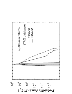
FIG. 1.: (a) $P(C_{ij})$ for C calculated using 30-min returns of 1000 stocks for the 2-yr period 1994–95 (solid line) and 881 stocks for the 2-yr period 1996–97 (dashed line). For the period 1996–97 $\langle C_{ij}\rangle=0.06$, larger than the value $\langle C_{ij}\rangle=0.03$ for 1994–95. The shaded region shows the distribution of correlation coefficients for the control $P(R_{ij})$ of Eq. (5), which is consistent with a Gaussian distribution with zero mean. (b) $P(C_{ij})$ calculated from daily returns of 422 stocks for five 7-yr sub-periods in the 35 years 1962–96. We find a large value of $\langle C_{ij}\rangle=0.18$ for the period 1983–89, compared with the average $\langle C_{ij}\rangle=0.10$ for the other periods.

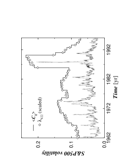
FIG. 2.: The stair-step curve shows the average value of the correlation coefficients $\langle C_{ij}\rangle$, calculated from $422\times 422$ correlation matrices C constructed from daily returns using a sliding $L=965$ day time window in discrete steps of $L/5=193$ days. The diamonds correspond to the largest eigenvalue $\lambda_{422}$ (scaled by a factor $4\times 10^{2}$) for the correlation matrices thus obtained. The bottom curve shows the S&P 500 volatility (scaled for clarity) calculated from daily records with a sliding window of length 40 days. We find that both $\langle C_{ij}\rangle$ and $\lambda_{422}$ have large values for periods containing the market crash of October 19, 1987.

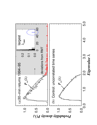
FIG. 3.: (a) Eigenvalue distribution $P(\lambda)$ for C constructed from the 30-min returns for 1000 stocks for the 2-yr period 1994–95. The solid curve shows the RMT result $P_{\rm rm}(\lambda)$ of Eq. (6). We note several eigenvalues outside the RMT upper bound $\lambda_{+}$ (shaded region). The inset shows the largest eigenvalue $\lambda_{1000}\approx 50\gg\lambda_{+}$. (b) $P(\lambda)$ for the random correlation matrix R, computed from $N=1000$ computer-generated random uncorrelated time series with length $L=6448$ shows good agreement with the RMT result, Eq. (6) (solid curve).

FIG. 4.: $P(\lambda)$ for C constructed from daily returns of 422 stocks for the 7-yr period 1990–96. The solid curve shows the RMT result $P_{\rm rm}(\lambda)$ of Eq. (6) using $N=422$ and $L=1,737$. The dot-dashed curve shows a fit to $P(\lambda)$ using $P_{\rm rm}(\lambda)$ with $\lambda_{+}$ and $\lambda_{-}$ as free parameters. We find similar results as found in Fig. 3(a) for 30-min returns. The largest eigenvalue (not shown) has the value $\lambda_{422}=46.3$.

FIG. 5.: (a) Nearest-neighbor (nn) spacing distribution $P_{\rm nn}(s)$ of the unfolded eigenvalues $\xi_{i}$ of C constructed from 30-min returns for the 2-yr period 1994–95. We find good agreement with the GOE result $P_{\rm GOE}(s)$ [Eq. (11)] (solid line). The dashed line is a fit to the one parameter Brody distribution $P_{\rm Br}$ [Eq. (12)]. The fit yields $\beta=0.99\pm 0.02$, in good agreement with the GOE prediction $\beta=1$. A Kolmogorov-Smirnov test shows that the GOE is $10^{5}$ times more likely to be the correct description than the Gaussian unitary ensemble, and $10^{20}$ times more likely than the GSE. (b) Next-nearest-neighbor (nnn) eigenvalue spacing distribution $P_{\rm nnn}(s)$ of C compared to the nearest-neighbor spacing distribution of GSE shows good agreement. A Kolmogorov-Smirnov test cannot reject the hypothesis that $P_{\rm GSE}(s)$ is the correct distribution at the 65% confidence level. The results shown above are using the Gaussian broadening procedure. Using the second procedure of fitting $F(\lambda)$ (Appendix A) yields similar results.

FIG. 6.: Nearest-neighbor spacing distribution $P(s)$ of the unfolded eigenvalues $\xi_{i}$ of C computed from the daily returns of 422 stocks for the 7-yr periods (a) 1962–68 (b) 1976–82 (c) 1983–89, and (d) 1990–96. We find good agreement with the GOE result (solid curve). The unfolding was performed by using the procedure of fitting the cumulative distribution of eigenvalues (Appendix A). Gaussian broadening procedure also yields similar results.

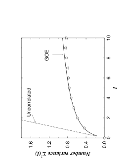
FIG. 7.: (a) Number variance $\Sigma^{2}(\ell)$ calculated from the unfolded eigenvalues $\xi_{i}$ of C constructed from 30-min returns for the 2-yr period 1994–95. We used Gaussian broadening procedure with the broadening parameter $a=15$. We find good agreement with the GOE result of Eq. 15 (solid curve). The dashed line corresponds to the uncorrelated case (Poisson). For the range of $\ell$ shown, unfolding by fitting also yields similar results.

FIG. 8.: (a) Distribution $\rho(u)$ of eigenvector components for one eigenvalue in the bulk $\lambda_{-}<\lambda<\lambda_{+}$ shows good agreement with the RMT prediction of Eq. (19) (solid curve). Similar results are obtained for other eigenvalues in the bulk. $\rho(u)$ for (b) u⁹⁹⁶ and (c) u⁹⁹⁹, corresponding to eigenvalues larger than the RMT upper bound $\lambda_{+}$ (shaded region in Fig. 3). (d) $\rho(u)$ for u¹⁰⁰⁰ deviates significantly from the Gaussian prediction of RMT. The above plots are for C constructed from 30-min returns for the 2-yr period 1994–95. We also obtain similar results for C constructed from daily returns.

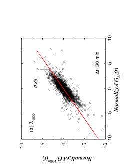
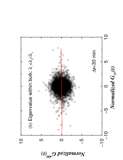
FIG. 9.: (a) S&P 500 returns at $\Delta t=30$ min regressed against the 30-min return on the portfolio $G^{1000}$ (Eq. (20)) defined by the eigenvector u¹⁰⁰⁰, for the 2-yr period 1994–95. Both axes are scaled by their respective standard deviations. A linear regression yields a slope $0.85\pm 0.09$. (b) Return (in units of standard deviations) on the portfolio defined by an eigenvector corresponding to an eigenvalue $\lambda_{400}$ within the RMT bounds regressed against the normalized returns of the S&P 500 index shows no significant dependence. Both axes are scaled by their respective standard deviations. The slope of the linear fit is $0.014\pm 0.011$, close to $0$ indicating that the dependence between $G^{1000}$ and $G_{\rm SP}(t)$ found in part (a) is statistically significant.

FIG. 10.: Probability distribution $P(C_{ij})$ of the cross-correlation coefficients for the 2-yr period 1994–95 before and after removing the effect of the largest eigenvalue $\lambda_{1000}$. Note that removing the effect of $\lambda_{1000}$ shifts $P(C_{ij})$ toward a smaller average value $\langle C_{ij}\rangle=0.002$ compared to the original value $\langle C_{ij}\rangle=0.03$.

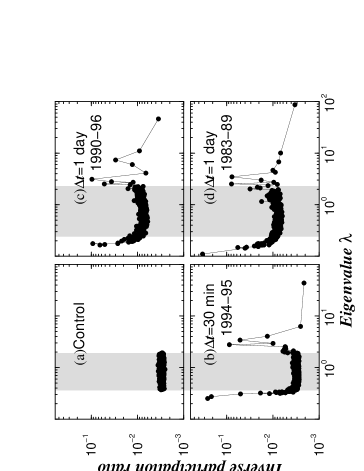
FIG. 11.: (a) Inverse participation ratio (IPR) as a function of eigenvalue $\lambda$ for the random cross-correlation matrix R of Eq. (6) constructed using $N=1000$ mutually uncorrelated time series of length $L=6448$. IPR for C constructed from (b) 6448 records of 30-min returns for 1000 stocks for the 2-yr period 1994–95, (c) 1737 records of 1-day returns for 422 stocks in the 7-yr period 1990–96, and (d) 1737 records of 1-day returns for 422 stocks in the 7-yr period 1983–89. The shaded regions show the RMT bounds $[\lambda_{+},\lambda_{-}]$.

FIG. 12.: All $10^{3}$ eigenvector components of u⁹⁹⁹ plotted against market capitalization (in units of US Dollars) shows that firms with large market capitalization contribute significantly. The straight line, which shows a logarithmic fit, is a guide to the eye.

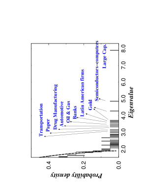
FIG. 13.: Schematic illustration of the interpretation of the eigenvectors corresponding to the eigenvalues that deviate from the RMT upper bound. The dashed curve shows the RMT result of Eq. (6).

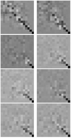
FIG. 14.: Grey scale pixel representation of the overlap matrix O$(t,\tau)$ as a function of time for 30-min data for the 2-yr period 1994–95. Here, the grey scale coding is such that black corresponds to $O_{ij}=1$ and white corresponds to $O_{ij}=0$. The length of the time window used to compute C is $L=1612$ ($\approx$60 days) and the separation $\tau=L/4=403$ used to calculate successive $O_{ij}$. Thus, the left figure on the first row corresponds to the overlap between the eigenvector from the starting $t=0$ window and the eigenvector from time window $\tau=L/4$ later. The right figure is for $\tau=2L/4$. In the same way, the left figure on the second row is for $\tau=3L/4$, the right figure for $\tau=4L/4$, and so on. Even for large $\tau\approx 1$ yr, the largest four eigenvectors show large values of $O_{ij}$.

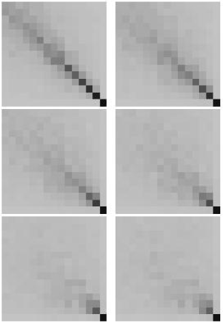
FIG. 15.: Grey scale pixel representation of the overlap matrix $\langle$O$(t,\tau)\rangle_{t}$ for 1-day data, where we have averaged over all starting points $t$. Here, the length of the time window used to compute C is $L=965$ ($\approx$4 yr) and the separation $\tau=L/5=193$ days used to calculate $O_{ij}$. Thus, the left figure on the first row is for $\tau=L/5$ and the right figure is for $\tau=2L/5$. In the same way, the left figure on the second row is for $\tau=3L/5$, the right figure for $\tau=4L/5$, and so on. Even for large $\tau\approx 20$ yr, the largest two eigenvectors show large values of $O_{ij}$.

FIG. 16.: (a) Portfolio return $R$ as a function of risk $D^{2}$ for the family of optimal portfolios (without a risk-free asset) constructed from the original matrix C. The top curve shows the predicted risk $D_{\rm p}^{2}$ in 1995 of the family of optimal portfolios for a given return, calculated using 30-min returns for 1995 and the correlation matrix C₉₄ for 1994. For the same family of portfolios, the bottom curve shows the realized risk $D_{\rm r}^{2}$ calculated using the correlation matrix C₉₅ for 1995. These two curves differ by a factor of $D_{\rm r}^{2}/D_{\rm p}^{2}\approx 2.7$. (b) Risk-return relationship for the optimal portfolios constructed using the filtered correlation matrix C^′. The top curve shows the predicted risk $D_{\rm p}^{2}$ in 1995 for the family of optimal portfolios for a given return, calculated using the filtered correlation matrix C${}^{\prime}_{94}$. The bottom curve shows the realized risk $D_{\rm r}^{2}$ for the same family of portfolios computed using C${}^{\prime}_{95}$. The predicted risk is now closer to the realized risk: $D_{\rm r}^{2}/D_{\rm p}^{2}\approx 1.25$. For the same family of optimal portfolios, the dashed curve shows the realized risk computed using the original correlation matrix C₉₅ for which $D_{\rm r}^{2}/D_{\rm p}^{2}\approx 1.3$.

FIG. 17.: (a) Autocorrelation function $c^{(k)}(\tau)$ of the time series defined by the eigenvector u⁹⁹⁹. The solid line shows a fit to a power-law functional form $\tau^{-\gamma_{k}}$, whereby we obtain values $\gamma_{k}=0.61\pm 0.06$. (b) To quantify the exponents $\gamma_{k}$ for all $k=1,\dots,1000$ eigenvectors, we use the method of DFA analysis [60] often used to obtain accurate estimates of power-law correlations. We plot the detrended fluctuation function $F(\tau)$ as a function of the time scale $\tau$ for each of the $1000$ time series. Absence of long-range correlations would imply $F(\tau)\sim\tau^{0.5}$, whereas $F(\tau)\sim\tau^{\nu}$ with $0.5<\nu\leq 1$ implies power-law decay of the correlation function with exponent $\gamma=2-2\nu$. We plot the exponents $\nu$ as a function of the eigenvalue and find values exponents $\nu$ significantly larger than $0.5$ for all the deviating eigenvectors. In contrast, for the remainder of the eigenvectors, we obtain the mean value $\nu=0.44\pm 0.04$, comparable to the value $\nu=0.5$ for the uncorrelated case.

REFERENCES

- [1] J. D. Farmer, Comput. Sci. Eng. 1, 26 (1999).
- [2] R. N. Mantegna and H. E. Stanley, An Introduction to Econophysics: Correlations and Complexity in Finance (Cambridge University Press, Cambridge 1999).
- [3] J. P. Bouchaud and M. Potters, Theory of Financial Risk (Cambridge University Press, Cambridge 2000).
- [4] J. Campbell, A. W. Lo, A. C. MacKinlay, The Econometrics of Financial Markets (Princeton University Press, Princeton, 1997).
- [5] E. P. Wigner, Ann. Math. 53, 36 (1951); Proc. Cambridge Philos. Soc. 47 790 (1951).
- [6] E. P. Wigner, “Results and theory of resonance absorption,” in Conference on Neutron Physics by Time-of-flight (Oak Ridge National Laboratories Press, Gatlinburg, Tennessee, 1956), pp. 59.
- [7] E. P. Wigner, Proc. Cambridge Philos. Soc. 47, 790 (1951).
- [8] F. J. Dyson, J. Math. Phys. 3, 140 (1962).
- [9] F. J. Dyson and M. L. Mehta, J. Math. Phys. 4, 701 (1963).
- [10] M. L. Mehta and F. J. Dyson, J. Math. Phys. 4, 713 (1963).
- [11] M. L. Mehta, Random Matrices (Academic Press, Boston, 1991).
- [12] T. A. Brody, J. Flores, J. B. French, P. A. Mello, A. Pandey, and S. S. M. Wong, Rev. Mod. Phys. 53, 385 (1981).
- [13] T. Guhr, A. Müller-Groeling, and H. A. Weidenmüller, Phys. Rep. 299, 190 (1998).
- [14] L. Laloux, P. Cizeau, J.-P. Bouchaud and M. Potters, Phys. Rev. Lett. 83, 1469 (1999).
- [15] V. Plerou, P. Gopikrishnan, B. Rosenow, L. A. N. Amaral, and H. E. Stanley, Phys. Rev. Lett. 83, 1471 (1999).
- [16] R. N. Mantegna, Eur. Phys. J. B 11, 193 (1999); L. Kullmann, J. Kertész, and R. N. Mantegna, e-print cond-mat/0002238; An interesting analysis of cross-correlation between stock market indices can be found in G. Bonanno, N. Vandewalle, R. N. Mantegna, e-print cond-mat/0001268.
- [17] P. Gopikrishnan, B. Rosenow, V. Plerou, and H. E. Stanley, Physical Review E, in press; See also cond-mat/0011145.
- [18] The time series of prices have been adjusted for stock splits and dividends.
- [19] Only those stocks, which have survived the 2-yr period 1994–95 were considered in our analysis.
- [20] V. Plerou, P. Gopikrishnan, L. A. N. Amaral, M. Meyer, and H. E. Stanley, Phys. Rev. E 60, 6519 (1999); P. Gopikrishnan, V. Plerou, L. A. N. Amaral, M. Meyer, and H. E. Stanley, Phys. Rev. E 60, 5305 (1999); P. Gopikrishnan, M. Meyer, L.A.N. Amaral, and H. E. Stanley, Eur. Phys. J. B 3, 139 (1998).
- [21] T. Lux, Applied Financial Economics 6, 463 (1996).
- [22] R. Muirhead, Aspects of Multivariate Statistical Theory (Wiley, New York, 1982).
- [23] F. J. Dyson, Revista Mexicana de Física, 20, 231 (1971).
- [24] A. M. Sengupta and P. P. Mitra, Phys. Rev. E 60 (1999) 3389.
- [25] M. J. Bowick and E. Brézin, Phys. Lett. B 268, 21, (1991); J. Feinberg and A. Zee, J. Stat. Phys. 87, 473 (1997).
- [26] Analytical evidence for this “universality” is summarized in Section 8 of Ref. [13].
- [27] A recent review is J. J. M. Verbaarschot and T. Wettig, e-print hep-ph/0003017.
- [28] For GOE matrices, the Wigner surmise (Eq. (11)) is not exact [11]. Despite this fact, the Wigner surmise is widely used because the difference between the exact form of and Eq. (11) is almost negligible [11].
- [29] Analogous to the GOE, which is defined on the space of real symmetric matrices, one can define two other ensembles [11]: (i) the Gaussian unitary ensemble (GUE), which is defined on the space of hermitian matrices, with the requirement that the joint probability of elements is invariant under unitary transformations, and (ii) the Gaussian symplectic ensemble (GSE), which is defined on the space of hermitian “self-dual” matrices with the requirement that the joint probability of elements is invariant under symplectic transformations. Formal definitions can be found in Ref. [11].
- [30] S. Drozdz, F. Gruemmer, F. Ruf, J. Speth, e-print cond-mat/9911168.
- [31] W. Sharpe, Portfolio Theory and Capital Markets (McGraw Hill, New York, NY, 1970).
- [32] W. Sharpe, G. Alexander, and J. Bailey, Investments, 5th Edition (Prentice-Hall, Englewood Cliffs, 1995).
- [33] W. Sharpe, J. Finance 19, 425 (1964).
- [34] J. Lintner, Rev. Econ. Stat. 47, 13 (1965).
- [35] S. Ross, J. Econ. Theory 13, 341 (1976).
- [36] S. Brown and M. Weinstein, J. Finan. Econ. 14, 491 (1985).
- [37] F. Black, J. Business 45, 444 (1972).
- [38] M. Blume and I. Friend, J. Finance 28, 19 (1973).
- [39] E. Fama and K. French, J. Finance 47, 427 (1992); J. Finan. Econ. 33, 3 (1993).
- [40] E. Fama and J. Macbeth, J. Political Econ. 71, 607 (1973).
- [41] R. Roll and S. Ross, J. Finance 49, 101 (1994).
- [42] N. Chen, R. Roll, and S. Ross, J. Business 59, 383 (1986).
- [43] R. C. Merton, Econometrica 41, 867 (1973).
- [44] B. Lehmann and D. Modest, J. Finan. Econ. 21, 213 (1988).
- [45] J. Campbell, J. Political Economy 104, 298 (1996).
- [46] J. Campbell and J. Ammer, J. Finance 48, 3 (1993).
- [47] G. Connor and R. Korajczyk, J. Finan. Econom. 15, 373 (1986); ibid. 21, 255 (1988); J. Finance 48, 1263 (1993).
- [48] A non-Gaussian one-factor model and its relevance to cross-correlations is investigated in P. Cizeau, M. Potters, and J.-P. Bouchaud, e-print cond-mat/0006034.
- [49] The limitations of a one-factor description as regards extreme market fluctuations can be found in F. Lillo and R. N. Mantegna, e-print cond-mat/0006065; e-print cond-mat/0002438.
- [50] Y. V. Fyodorov and A. D. Mirlin, Phys. Rev. Lett. 69, 1093 (1992); 71, 412 (1993); Int. J. Mod. Phys. B 8, 3795 (1994); A. D. Mirlin and Y. V. Fyodorov, J. Phys. A: Math. Gen. 26, L551 (1993); E. P. Wigner, Ann. Math. 62, 548 (1955).
- [51] P. A. Lee and T. V. Ramakrishnan, Rev. Mod. Phys. 57, 287 (1985).
- [52] Metals or semiconductors with impurities can be described by Hamiltonians with random-hopping integrals [F. Wegner and R. Oppermann, Z. Physik B34, 327 (1979)]. Electron-hopping between neighboring sites is more probable than hopping over large distances, leading to a Hamiltonian that is a random band matrix.
- [53] Y. Liu, P. Gopikrishnan, P. Cizeau, C.-K. Peng, M. Meyer, and H. E. Stanley, Phys. Rev. E 60, 1390 (1999); Y. Liu, P. Cizeau, M. Meyer, C.-K. Peng, and H. E. Stanley, Physica A 245, 437 (1997); P. Cizeau, Y. Liu, M. Meyer, C.-K. Peng, and H. E. Stanley, Physica A 245, 441 (1997).
- [54] E. J. Elton and M. J. Gruber, Modern Portfolio Theory and Investment Analysis, J. Wiley, New York, 1995.
- [55] L. Laloux et al., Int. J. Theor. Appl. Finance 3, 391 (2000).
- [56] J. D. Noh, Phys. Rev. E 61, 5981 (2000).
- [57] M. Marsili, e-print cond-mat/0003241.
- [58] K. H. Fischer and J. A. Hertz, Spin Glasses (Cambridge University Press, New York, 1991).
- [59] J. D. Farmer, e-print adap-org/9812005; R. Cont and J.-P. Bouchaud, Eur. Phys. J. B 6, 543 (1998).
- [60] C. K. Peng, et al., Phys. Rev. E 49, 1685 (1994).
- [61] V. Plerou, P. Gopikrishnan, L. A. N. Amaral, X. Gabaix, and H. E. Stanley, Phys. Rev. E 62, R3023 (2000).
- [62] In contrast, the autocorrelation function for the S&P 500 index returns displays only correlations on short-time scales of min, beyond which the autocorrelation function is at the level of noise [53]. On the other hand, the returns for individual stocks have pronounced anti-correlations on short time scales ( min), which is an effect of the bid-ask bounce [4]. For certain portfolios of stocks, returns are found to have long memory [A. Lo, Econometrica 59, 1279 (1991)].
- [63] For the case of predominantly “ferromagnetic” couplings () within disjoint groups of stocks, a factor model (such as Eq. (21)) can be derived from the model of “interacting stocks” in Eq. (31). In the spirit of a mean-field approximation, the influence of the price changes of all other stocks in a group on the price of a given stock can be modeled by an effective field, which has to be calculated self-consistently. This effective field would then play a similar role as a factor in standard economic models.
- [64] M. Brack, J. Damgaard, A.S. Jensen, H.C. Pauli, V.M. Strutinsky, and C.Y. Wong, Rev. Mod. Phys. 44, 320 (1972).
- [65] H. Bruus and J.-C Anglés d’Auriac, Europhys. Lett. 35, 321 (1996).