Abstract

In this work we study a two species driven diffusive system with open boundaries that exhibits spontaneous symmetry breaking in one dimension. In a symmetry broken state the currents of the two species are not equal, although the dynamics is symmetric. A mean field theory predicts a sequence of two transitions from a strongly symmetry broken state through an intermediate symmetry broken state to a symmetric state. However, a recent numerical study has questioned the existence of the intermediate state and instead suggested a single discontinuous transition. In this work we present an extensive numerical study that supports the existence of the intermediate phase but shows that this phase and the transition to the symmetric phase are qualitatively different from the mean-field predictions.

1 Introduction

Nonequilibrium systems may be defined as systems evolving according to dynamics that are not constructed from any detailed balance condition. Thus their steady states are not described by Gibbs-Boltzmann statistical mechanics. In particular, such a steady state is characterised by nonvanishing currents of probability between configurations. These nonequilibrium steady states have been the subject of much attention for some years now and their properties are of fundamental interest [1]. For example, generic long-range correlations and nonequilibrium phase transitions, even in one dimension, may be exhibited [2, 3, 4]; such behaviour is in contrast to that of equilibrium steady states.

One class of nonequilibrium systems are driven diffusive systems (DDS). As well as probability currents existing these systems also have a mass current of a conserved quantity driven through the system. DDS lend themselves to the modelling of a variety of phenomena such as super-ionic conductors, traffic flow and biophysical transport problems [1, 2].

Perhaps the simplest DDS is the asymmetric simple exclusion process (ASEP). Here particles hop in a preferred direction on a one-dimensional lattice with hard-core exclusion (at most one particle can be at any given site). The open system where particles are injected and extracted at the boundaries was first studied by Krug[5] and boundary-induced phase transitions shown to be possible. Since then our understanding of phase transitions in one-dimensional DDS has deepened through exact solutions of this model being worked out [6]–[13] and further examples being studied. Of particular interest have been phase transitions manifesting spontaneous symmetry breaking [14, 15, 16, 17, 18], phase transitions and phase separation induced by defect particles or defect sites [19, 20, 21, 22, 23, 24], phase separation in multicomponent systems [25, 26] and further examples of boundary-induced phase transitions [27, 28]. Clearly the presence of conserved quantities and a drive, leading to non-zero current $j$ is crucial to all these phase transitions.

Exact results have provided us with a particularly good understanding of the ASEP with open boundary conditions. Let us summarise some of the results here. The open system is defined on a lattice of $N$ sites where at the left boundary a particle is introduced with rate $\alpha$ if that site is empty, and at the right boundary site any particle present is removed with rate $\beta$. These boundary conditions force a steady state current of particles $j_{N}$ through the system. Phase transitions occur when the current in the thermodynamic limit, $j=\lim_{N{\to}\infty}j_{N}$, exhibits non-analyticities. The steady state of this system was solved exactly first for the totally asymmetric hopping case [7, 8]. The phase diagram comprises three phases: a high-density phase where the system is controlled by the low exit rate $\beta$ ($\beta<1/2;\alpha>\beta)$, the current takes the value $j=\beta(1-\beta)$ and the bulk density is $\rho=(1-\beta)$; a low-density phase where the system is controlled by a low injection rate $\alpha$ ($\alpha<1/2;\alpha<\beta$), the current is $j=\alpha(1-\alpha)$ and the bulk density is $\rho=\alpha$; a maximal-current phase where both $\alpha,\beta>1/2$ and the current is $j=1/4$ and the bulk density $\rho=1/2$. The exact solution has been generalised to partially asymmetric hopping and retains the same three generic phases [11, 12]. Indeed, the qualitative phase diagram appears robust for one-dimensional, open, driven systems [29, 30].

The phase transitions from the high density or low density phases to the maximal-current phase are both continuous—the density is continuous at the transition but has a discontinuity in its first derivative and the current has a discontinuity in its second derivative. However the transition from the high density to the low density phase is discontinuous—the density is discontinuous and the current has a discontinuity in its first derivative at the transition. On the coexistence line between the high and low density phases the system consists of a low density region adjacent to the left boundary and a high density region adjacent to the right boundary. The currents within the two domains are equal (otherwise one phase would be driven out of the system) and domains are separated by a shock, i.e. a sharp domain wall that performs diffusive motion due to fluctuations in the number of particles entering and leaving the system [10].

The above observations suggest an analogy between the role of the current for a driven system and the role of the chemical potential in an equilibrium system. That is, whereas in equilibrium the condition for phase coexistence is that the chemical potential of the two phases must be equal, in the present case one must have that the currents in the two phases are equal. Indeed, the exact solution [7] revealed that the current is expressed as the ratio of partition sums for systems of size $N{-}1$ and $N$ yielding an explicit identification of $j$ as a fugacity (i.e. the exponential of a chemical potential).

A further kind of boundary-induced phase transition, manifesting spontaneous symmetry breaking, is found when the model is generalised to two oppositely moving species of particle: one species is injected at the left, moves rightwards and exits at the right; the other species is injected at the right, moves leftwards and exits at the left [14]. Intuitively one can picture the system as a narrow road bridge: cars moving in opposite directions can pass each other but cannot occupy the same space. The model has a left-right symmetry when the injection rates and exit rates for the two species of particles are symmetric. However for low exit rates ($\beta$) this symmetry is broken and the lattice is dominated by one of the species at any given time. This implies that the short time averages of currents and bulk densities of the two species of particles are no longer equal. Over longer times the system flips between the two symmetry-related states. In the $\beta\to 0$ limit the mean flip time between the two states has been calculated analytically and shown to diverge exponentially with system size [15]. Thus the ‘bridge’ model provided a first example of spontaneous symmetry breaking in a one dimensional system.

Of particular interest is the transition from the low $\beta$ regime where the symmetry is broken to the high $\beta$ regime where the steady state is symmetric. A mean-field theory [14](to be reviewed in section 2.1) predicts the following scenario in terms of the phases of the single species model. For low $\beta$ one species of particles (the dominant one) is in a high density phase whereas the other is in a low density phase. This will be referred to as the hd/ld phase. As $\beta$ is increased a discontinuous transition occurs to another asymmetric phase where both particles are in single species low density phases (ld/ld phase) i.e. the density of each species is less than 1/2 but the densities are different. As $\beta$ is increased further a continuous transition occurs to a symmetric phase wherein the species have the same density with value less than 1/2 (ld phase).

Thus, in this scenario, there is a sequence of two transitions with the ld/ld phase appearing as the intermediate phase. The intermediate phase occupies a very narrow region of the mean field phase diagram, nevertheless in [14], Monte Carlo simulations provided some evidence supporting its existence.

However, Arndt et al [16] have argued on the basis of numerical studies that there is a single discontinuous transition and that the ld/ld phase does not exist. In order to draw their conclusions Arndt et al used the concept of a nonequilibrium free energy. This simply involves calculating the probability distribution of the particle densities in the steady state. Arndt et al then converted this into a ‘free energy density’ as a function of particle densities by taking the logarithm of the distribution and dividing by $N$.

In order to clarify the discrepancy between the results of [14] and [16] we further investigate in this work the transition from the asymmetric state to the symmetric state. We present extensive numerical studies and theoretical arguments that suggest that the intermediate ld/ld phase does indeed exist. However, our numerics indicate that the sequence of transitions is distinct from both the mean-field prediction and the scenario proposed in [16]. Instead, we observe a third scenario in which as $\beta$ is increased a discontinuous transition occurs from the hd/ld to the ld/ld phase, then a further discontinuous transition occurs from the ld/ld to the symmetric phase.

The two first order transitions displayed by this model are found to be of a different nature. In the transition between the hd/ld and the ld/ld phases, the two phases have the same currents, and thus they may coexist in the same system with one fraction of the system occupied by one phase and the rest of the system by the other. This is closely analogous to ordinary first order transitions in equilibrium where the phases involved in the transition have the same chemical potential. On the other hand the first order transition from the asymmetric ld/ld to the symmetric phase is found to be of a different nature, which has no equilibrium analogue. Here the currents of the two phases are not equal to each other and thus the two phases cannot coexist in the same system for a long time.

The layout of the paper is as follows. In Section 2 we define the model and review the mean-field theory. In Section 3 our numerical simulations are presented, in particular we provide numerical evidence for two discontinuous transitions. In Section 4 we discuss a simplistic ‘blockage’ picture that captures some features of the simulations. In Section 5 we conclude and resolve the discrepancies between our conclusions and those of [16].

2 Model definition and mean-field theory

We now define the bridge model described in the introduction. We indicate the presence of a hole by ‘0’, and of a positive or negative particle by ‘$+$’ and ‘$-$’ respectively. The site is denoted by an index. The possible configuration changes that may occur in time $\mathrm{d}t$ can be described as follows:

left end:

$$\begin{array}[]{lcl}(0)_{1}\to(+)_{1}&\mbox{with probability}&\alpha\;\mbox{d}t\\[4.30554pt] (-)_{1}\to(0)_{1}&\mbox{with probability}&\beta\;\mbox{d}t\end{array}$$ (1)

right end:

$$\begin{array}[]{lcl}(0)_{N}\to(-)_{N}&\mbox{with probability}&\alpha\;\mbox{d}t\\[4.30554pt] (+)_{N}\to(0)_{N}&\mbox{with probability}&\beta\;\mbox{d}t\end{array}$$ (2)

bulk ($1<i<N$):

$$\begin{array}[]{lcl}(+)_{i}(0)_{i+1}\to(0)_{i}(+)_{i+1}&\mbox{with probability}&\mbox{d}t\\[4.30554pt] (0)_{i}(-)_{i+1}\to(-)_{i}(0)_{i+1}&\mbox{with probability}&\mbox{d}t\\[4.30554pt] (+)_{i}(-)_{i+1}\to(-)_{i}(+)_{i+1}&\mbox{with probability}&\mbox{d}t\end{array}$$ (3)

Thus the two types of particles—referred to as ‘positive’ and ‘negative’ particles although they exhibit only hard-core interaction—hop with rate 1 in opposite directions on a lattice of $N$ sites. Positive particles are injected at the left-hand side with rate $\alpha$, if the first site is empty, and removed from the right-hand boundary with rate $\beta$ if the last site is occupied. With respect to the two types of particles the model is symmetric, thus negative particles enter the system on the right-hand side with rate $\alpha$, and leave on the left-hand side with rate $\beta$.

In the following we will consider only the case $\alpha=1$.

2.1 Mean-field theory

Here we review the mean-field theory and associated phases [14]. The mean-field theory is implemented by approximating two-point correlation functions by products of one-point correlations functions.

Let $p_{i}$ ($m_{i}$) denote the average positive (negative) particle density at site $i\in\{1,2,...,N\}$. In a stationary state, the positive (negative) particle currents $j^{+}$ ($j^{-}$) through the system are site independent and satisfy, in the mean-field theory,

$$j^{+} = p_{i}\left(1-p_{i+1}\right)$$ (4)

$$j^{-} = m_{i+1}\left(1-m_{i}\right)$$ (5)

for the bulk ($1<i<N$) and

$$j^{+} = \left(1-p_{1}-m_{1}\right)=\beta p_{N}$$ (6)

$$j^{-} = \beta m_{1}=\left(1-p_{N}-m_{N}\right)$$ (7)

for the boundaries. We will denote the limiting bulk densities far away from the boundaries as $p,m$ so that in the limit of large $N$

$$j^{+} \to p\left(1-p\right)$$ (8)

$$j^{-} \to m\left(1-m\right)\;.$$ (9)

Notice that the two systems of particles are only coupled by the boundary conditions (6,7). The mean-field theory solves for the currents through the definition of effective boundary rates

$$\alpha^{+} = \frac{1-p_{1}-m_{1}}{1-p_{1}}=\frac{j^{+}}{j^{+}+j^{-}/\beta}$$ (10)

$$\alpha^{-} = \frac{1-p_{N}-m_{N}}{1-m_{N}}=\frac{j^{-}}{j^{-}+j^{+}/\beta}$$ (11)

$$\beta^{+} = \beta^{-}=\beta$$ (12)

Then the equations for the currents of each species can be solved self-consistently by using the solutions of the mean-field theory for the single species model [6].

Depending on the feeding and output rates $\alpha^{S}$ and $\beta^{S}$ (superscript “S” denoting the single species quantities) there exist three different phases in the single species model:

• The maximal-current or power-law phase with current $j^{S}=1/4$ for $\alpha^{S}\geq 1/2$ and $\beta^{S}\geq 1/2$. The bulk density is $1/2$, the density profile obeys a power law.

• The low-density phase for $\alpha^{S}<\beta^{S}$ and $\alpha^{S}<1/2$. The current is $j^{S}=\alpha^{S}(1-\alpha^{S})$ and the bulk density is equal to $\alpha^{S}$.

• The high-density phase for $\beta^{S}<\alpha^{S}$ and $\beta^{S}<1/2$. The current is $j^{S}=\beta^{S}(1-\beta^{S})$ and the bulk density equals $1-\beta^{S}$.

Considerations concerning which of these phases are compatible with each other lead to the identification of four phases for the two species system[14].

• Symmetric phases: in these phases $j^{+}=j^{-}$, hence from (10,11)

  $$\alpha^{S}=\alpha^{+}=\alpha^{-}=\frac{\beta}{1+\beta}$$ (13)

  • Maximal Current symmetric phase: both species are in the maximal single species phase. Thus $j^{+}=j^{-}=1/4$ and $p=m=1/2$. The phase exists for $\alpha^{S}\geq 1/2$ which corresponds to $\beta\geq 1$.

  • Low-density symmetric phase: both species are in the low density single species phase. Thus $j^{+}=j^{-}=\beta/(1+\beta)^{2}$ and $p=m=\beta/(1+\beta)$. The phase exists for $\beta\leq 1$.

• Asymmetric phases: in these phases $j^{+}\neq j^{-}$ (it will be assumed that the positive particles are the majority species i.e. $j^{+}>j^{-}$):

  • High-density/low-density phase: positive particles are in a high density phase and negative particles in a low density phase thus

    $$j^{+} = \beta\left(1-\beta\right)$$ (14)

    $$j^{-} = \alpha^{-}\left(1-\alpha^{-}\right)$$ (15)

    where

    $$\alpha^{-}=1-\sqrt{1-\beta}\;.$$ (16)

    The bulk densities are

    $$p=1-\beta\quad\mbox{and}\quad m=1-\sqrt{1-\beta}\;.$$ (17)

    This phase is found for $\alpha^{+}>\beta$ which yields using (10, 14,15) $\beta<0.329$

  • Low-density/low-density asymmetric phase: positive particles and negative particles are in distinct low density phases thus

    $$j^{+} = \alpha^{+}\left(1-\alpha^{+}\right)$$ (18)

    $$j^{-} = \alpha^{-}\left(1-\alpha^{-}\right)$$ (19)

    where $\alpha^{+}\neq\alpha^{-}$. Some calculation yields for the densities

    $$p=\alpha^{+} = \frac{1}{2(1-\beta)}\left[(1-2\beta)+\left(\frac{1-3\beta}{1+\beta}\right)^{1/2}\right]$$ (20)

    $$m=\alpha^{-} = \frac{1}{2(1-\beta)}\left[(1-2\beta)-\left(\frac{1-3\beta}{1+\beta}\right)^{1/2}\right]$$ (21)

    The condition for this phase is $\alpha^{+}<\beta$ i.e. $\beta<0.329$. There is a continuous transition to the ld symmetric phase at $\beta=1/3$

Thus, as we increase $\beta$ from zero the mean-field theory predicts the following sequence of transitions: at $\beta=0.329$ a discontinuous transition from hd/ld to ld/ld; at $\beta=1/3$ a continuous transition from the ld/ld asymmetric to the low-density symmetric phase; at $\beta=1$ a continuous transition from the ld phase to the maximal current phase.

3 Simulations

We have carried out various numerical simulations to investigate the transition from the hd/ld to the ld symmetric phase to gain some insight into whether a second asymmetric phase is present. A standard random sequential updating procedure is used to simulate the dynamics Eqns. (1–3).

First of all, we followed the idea of Arndt et al [16] and simulated the probability distribution $P(p,m)$ of the steady state as a function of both positive and negative particle density $p$ and $m$ and for various $\beta$. In a simulation the positive and negative particle densities $p$ and $m$ are evaluated every ten Monte Carlo steps to built up a histogram for the probability distribution $P(p,m)$.

As shown in Figures 1 to 5 where $P(p,m)$ is plotted for a system size of $N=500$ sites and $\beta=0.265,0.274,0.280,0.284$ and $0.290$ the three different phases qualitatively predicted by mean-field theory can be found. Quantitatively, the values differ from the mean-field results which predict the transition from the hd/ld to the ld/ld for $\beta=0.329$ and the transition to the symmetric phase for $\beta=1/3$.

Figure 1: A 3-d plot of the probability density $P(p,m)$ as a function of the particle densities $m,p$ for $N=500$, $\beta=0.265$. A contour plot is shown projected onto the $m-p$ plane.

Figure 2: $P(p,m)$ as in Fig. 1 for $N=500$, $\beta=0.274$, different scale than Figures 1, 3–5

Figure 3: $P(p,m)$ as in Fig. 1 for $N=500$, $\beta=0.280$

Figure 4: $P(p,m)$ as in Fig. 1 for $N=500$, $\beta=0.284$

Figure 5: $P(p,m)$ as in Fig. 1 for $N=500$, $\beta=0.290$

In Fig. 1 $\beta=0.265$ and the system is in the hd/ld phase. The probability distribution shows two well-separated peaks at $(p,m)\approx(0.74,0.14)$ and $(p,m)\approx(0.14,0.74)$ which correspond to the densities $\rho_{\rm majority}=1-\beta$ and $\rho_{\rm minority}=1-\sqrt{1-\beta}$ predicted by mean-field theory in section 2.1. A transition occurs at $\beta\approx 0.274$ (Fig. 2). One observes the ‘boomerang’ shape described by Arndt et al : in the two arms of the boomerang of the probability distribution the density of one particle type is constant and the density of the other fluctuates strongly. This behaviour corresponds to coexistence of the hd/ld and ld/ld phases in the same system with a wandering domain wall or shock that is equally likely to be at any position separating the regions of different density. However, there is a clear saddle point separating the two arms of the boomerang. This is in contrast to the first order transition proposed by Arndt et al. in which $P(p,m)$ is supposed to be constant along the whole structure. At $\beta=0.280$ (Fig. 3), we observe evidence for a ld/ld asymmetric phase. The probability distribution shows two peaks at values which are $<1/2$ for both $p$ and $m$ confirming the existence of a ld/ld asymmetric phase. However note that the saddle point separating the two peaks itself has a high probability. When $\beta$ is increased to 0.284 (Fig. 4) the probability appears to have a flat top indicating that one is at the transition to the symmetric phase. Finally, For $\beta=0.29$ the system is in the symmetric phase with $p=m=0.22\simeq\beta/(1+\beta)$.

The maxima in the probability distribution, corresponding to a second symmetry broken phase, are clearly visible for $\beta=0.280$, but there remain some questions about the nature of this ld/ld phase. First of all, the location of the peaks is not correctly described by mean-field theory; the minority density is $\rho_{\rm minority}\simeq 1-\sqrt{1-\beta}$ as for the hd/ld phase, but the majority species is found to be present with density $\rho_{\rm majority}\simeq\beta$ which does not agree with the mean-field value. Furthermore, it is striking that the maxima are not only separated by a very high saddle, but also have long tails in the hd/ld region of the distribution that are a vestige of the transition from the hd/ld phase (Fig. 2).

To gain a deeper understanding of these features, we explicitly illustrate the time evolution of the densities at $\beta=0.275$ close to the transition from the hd/ld phase (Figs. 6–8). The sequence shows different periods of a single simulation run. The positive and negative particle densities $p$ and $m$ and their difference are plotted. Different types of behaviour are clearly observed as time evolves. In Fig. 6 the simulation begins with densities corresponding to the arm of the boomerang: the density of the majority phase fluctuates strongly, while that of the minority phase is relatively constant. In Fig. 7 the simulation moves into a short period of symmetric densities corresponding to the ld phase then progresses to a symmetry broken period corresponding to the ld/ld phase. Finally Figure 8 illustrates curious oscillations in the densities about the symmetric value that can sometimes be observed.

Thus in the ld/ld region there appear to be different behaviours competing for the true phase behaviour. One might expect this to be a finite size effect and that for $N\to\infty$ one behaviour dominates. We will provide evidence for this below.

Another consequence of competing behaviours is that they do not coexist in a system, rather the system switches from one behaviour to another. This implies that although the transition to from the ld/ld phase to the symmetric is discontinous there is no coexistence between the phases. This is in contrast to the discontinous transition from the hd/ld to the ld/ld phase where there is coexistence. One can also rule out coexistence at the ld/ld to symmetric phase transition on theoretical grounds: it is not possible for a phase with symmetric currents to coexist with a phase with asymmetric currents in the same system. Curiously, although coexistence does not occur, figure 4, appears to have a flat-topped distribution. It would be interesting to see whether this is just a finite size effect.

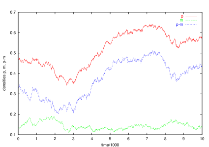
Figure 6: Time evolution of the particle densities $p$, $m$ and density difference $p-m$ during a single simulation at $\beta=0.275$: minority species has low density $\rho_{\rm min}=1-\sqrt{1-\beta}\simeq 0.149$, density of majority species fluctuates strongly

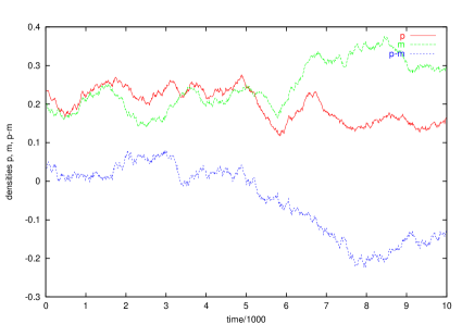
Figure 7: Time evolution of the particle densities $p$, $m$ and density difference $p-m$ during a single simulation at $\beta=0.275$: weak fluctuations around $\rho_{\rm sym}=\frac{\beta}{1+\beta}=0.216$ turn into asymmetric phase with $\rho_{\rm min}\simeq 1-\sqrt{1-\beta}=0.149$ and $\rho_{\rm maj}\simeq\beta=0.275$

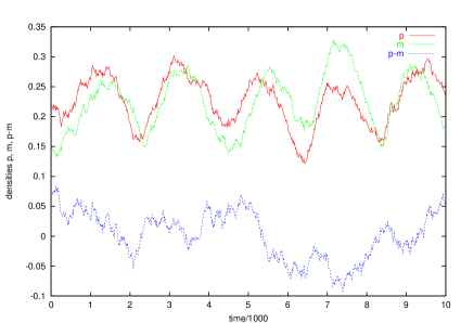
Figure 8: Time evolution of the particle densities $p$, $m$ and density difference $p-m$ during a single simulation at $\beta=0.275$: both species fluctuate strongly around density value of symmetric phase $\rho_{\rm sym}=\frac{\beta}{1+\beta}=0.216$

We defer the introduction of a more intuitive description than mean-field theory, which will explain some of the findings described above, to the next section. We first have a closer look at how the behaviour near the transitions changes with increasing system size.

To provide a more convenient two-dimensional representation of $P(p,m)$, we will plot in the following the maximum of $P(p,m)$ as seen along diagonals satifying $p-m=constant$. As the probability distribution is symmetric around the $p=m$, it is sufficient to restrict the plot to $p-m>0$.

For increasing system size $N$, the peaks corresponding to a ld/ld asymmetric region become more pronounced as is shown in Figure 9 for system sizes of $N=100$—$2000$ and for an exit rate $\beta=0.275$. To quantify the sharpening of the peaks we plot the ratio of the height of the peak to the height of saddle

Figure 9: Maximum of $P(p,m)$ for $\beta=0.275$ and $N=100$, $200$, $500$, $1000$, $2000$

in Figure 10.

Figure 10: maximum/saddle ratio in the probability distribution $P(p,m)$

Although the increase is slow, it is monotonic and can be fitted by a power law ($\propto N^{0.12}$). This indicates that the peaks corresponding to a ld/ld phase should dominate the probability distribution in the large $N$ limit. Figure 10 thus provides strong evidence that the ld/ld phase does truly exist.

However, one should note that the power-law scaling of the peak to saddle ratio is unusual—within an equilibrium free energy picture (where $P(p,m)\sim\exp Nf(p,m)$) one would expect the ratio to scale exponentially with $N$. Conversely the power-law scaling implies that the escape time or flip time from the ld/ld phase does not increase exponentially with $N$. We will return to this point in the conclusion.

4 Blockage picture

In the previous section the simulations provided evidence for a ld/ld asymmetric phase but with values of the densities different from those predicted by mean-field theory. We also saw coexistence between the hd/ld and ld/ld phases at the transition.

Here we draw on the simulations to give a more intuitive description of the ld/ld phase that we will refer to as the blockage picture. This picture builds on observations of [14] and [16], the exact results for $\beta\to 0$ [15] and general theoretical considerations of [29, 30].

First we sketch the qualitative features of the hd/ld phase as predicted by mean-field theory and confirmed by the exact results for $\beta\to 0$. Schematically the instantaneous picture is as in Fig. 11 a): the bulk of the lattice is occupied by a blockage of positive particles. In the figure $p_{N}^{\rm bp}$ denotes the density of the majority species (travelling from left to right) in the blockage and $p_{1}^{\rm bp}$ denotes the density to the left of the blockage (the upper index ‘bp’ denotes blockage picture). Similarly $m_{1}^{\rm bp}$ denotes the density of the minority species near the left boundary and $m_{N}^{\rm bp}$ denotes the density away from the left boundary. Near the left boundary there is a small blockage of negative particles. This blockage is unstable in the sense that the domain wall between it and the bulk region drifts to the left. Averaging over the positions of the domain wall results in the exponential decay of the mean field density profile from the left boundary [29].

Figure 11: Schematic picture of the instantaneous density profiles in asymmetric phases with $p$ being the majority and $m$ being the minority species. a)High density/low density b) low density/low density

Now we summarise some important features of the ld/ld phase that we have observed in simulations. The simulations show that small blockages are formed by the majority species at its output end. This prevents the other particle species from entering and leads to the symmetry breaking. However for finite size systems these blockages are not stable for long times (at least not for times exponential in the system size) which contrasts with the hd/ld phase.

These observations lead us to the following blockage picture for the ld/ld phase as illustrated in Figure 11 b). There is a small blockage of positive particles at the right end of the system. Thus the domain wall of Figure 11 a) is now pushed to the right end of the system. In order to obtain the currents and the densities in the ld/ld phase we assume that the blockage of the majority species is stable in the sense that the current into the blockage equals the current out. We also assume that the the densities of both species are basically constant within each domain. This is backed up by our numerical results. This assumption of a stable blockage and constant density at the output side of the majority species implies using the mean-field equations (4–7) that

$$j^{+}=p_{N}^{\rm bp}(1-p_{N}^{\rm bp})=\beta p_{N}^{\rm bp}$$ (22)

thus

$$p_{N}^{\rm bp}=1-\beta\quad\mbox{and}\quad j^{+}=\beta(1-\beta)\;.$$ (23)

Since the current into the blockage is equal to the current out one obtains

$$p_{1}^{\rm bp}=\beta\;.$$ (24)

The blockage also controls the input of the minority species and we can determine $m_{N}^{\rm bp}$ from the condition

$$j^{-}=1-m_{N}^{\rm bp}-p_{N}^{\rm bp}=m_{N}^{\rm bp}(1-m_{N}^{\rm bp})$$ (25)

and one finds

$$m_{N}^{\rm bp}=1-\sqrt{1-\beta}\;.$$ (26)

Note that these results for the bulk densities (24,26) differ from the mean-field theory predictions (20,21). Also observe that (23,26) are the same as the corresponding mean-field expressions for the hd/ld phase (17). Thus one can think of the blockage picture as being an extension of the mean-field theory into the ld/ld regime. Finally observe that the majority and minority densities given by the blockage picture for the ld/ld phase do not coincide (except at $\beta=1$ or 0) thus the blockage picture is consistent with a discontinuous transition to the symmetric phase at some lower value of $\beta$.

To summarise, in the case of the hd/ld phase the blockage occupies the bulk of the system, the bulk density for the majority species is given by $\rho^{+}=p_{N}^{\rm bp}=1-\beta$. The bulk density for the minority species is given by $\rho^{-}=m_{N}^{\rm bp}=1-\sqrt{1-\beta}$. At the transition from the hd/ld to the ld/ld phase the domain wall may be found anywhere in the system. This corresponds to a shock, that is a sudden change in density over a microscopic region. The wandering of the shock produces the arms of the boomerang on the plots of $P(p,m)$ presented in Figure 2. In the ld/ld phase the domain wall is localised at the right end of the system. The bulk densities are given by (24,26) as $\rho^{+}=\beta$ and $\rho^{-}=1-\sqrt{1-\beta}$.

The blockage picture explains the qualitative features of the phases and predicts quantitatively the densities in the ld/ld phase. However, it does not make any further quantitative predictions e.g. for the values of $\beta$ at the transition points. Also some features remain unexplained. For example in the ld/ld phase a stable blockage (as defined above) is assumed at the right hand boundary. For such a blockage, one would expect a diffusive motion of the domain wall leading it to explore the whole system. Yet, this only occurs at the transition from hd/ld to ld/ld; in the ld/ld phase the blockage is pinned near that boundary. This suggests that the blockage is only stable over short times. It would be interesting to understand this more fully.

5 Conclusions

In this paper we studied a totally asymmetric simple exclusion process for two species which exhibits spontaneous symmetry breaking. In particular we have made a detailed study of the transition from the symmetry broken regime to the symmetric regime. We carried out Monte Carlo simulations to investigate the transition between the previously studied high-density/low density asymmetric phase [14, 15] and a symmetric phase. We found evidence for the existence of a second asymmetric phase. However although the observed particle densities in this region are unequal and both smaller than $1/2$, they do not correspond to the predictions of the mean-field ld/ld asymmetric phase.

Instead a simplistic description of this phase is provided by the ‘blockage picture’. It ascribes the symmetry breaking in the two species system to the buildup of blockages at the output end of one particle type due to the low output rate. These blockages then prevent the other particle species from entering which results in a lower density. This picture is in accord with mean-field theory for the hd/ld phase; it gives new insight into the observed ld/ld asymmetric phase.

Interestingly, although both transitions (from hd/ld to ld/ld and from ld/ld to symmetric) are discontinuous, they are of different types. At the first transition one has coexistence between the hd/ld and ld/ld phases. This is manifested by the presence of a shock in the density of the majority species wandering through the system. At the ld/ld to symmetric transition, however, one cannot have coexistence simply because a phase with symmetric currents of particles cannot coexist in the same system with a phase where the currents are not symmetric. Thus we have a discontinous transition without coexistence.

We now address the discrepancies between our conclusions and those of Arndt et al.

The approach of Arndt et al[16] is to assign a free energy density to the probability distribution of the steady states. It is defined as the negative logarithm of a probability distribution $P(p-m)$ which depends only on the density difference (and implicitly on the system size $N$):

$$f(p-m)=\lim_{N\to\infty}\left(-\frac{1}{N}\log{P(p-m)}\right)$$ (27)

However in that work $P(p-m)$ is calculated by integrating $P(p,m)$ along diagonals satisfying $p-m=constant$. $P(p-m)$ therefore does not distinguish between the rather narrow peaks and the lower but wider saddle between them. Considering the logarithm of this function to calculate the free energy will flatten any remaining maxima of $P(p-m)$ in the ld/ld phase even further. This explains why Arndt et al concluded the ld/ld phase was absent. In Fig. 9, on the other hand, we project $P(p,m)$ onto a two dimensional representation by taking the maximum along the diagonals $p-m=constant$. For the finite size systems considered this preserves more faithfully the three dimensional structure of $P(p,m)$ and we clearly see the ld/ld phase.

Finally, we would like to mention the flip time in the asymmetric phases. For finite system sizes the blockages in the ld/ld asymmetric phase are only stable for short times implying that the flip time in this asymmetric phase is in turn small. For $\beta$ vanishingly small (i.e. in the hd/ld phase) it is known that the flipping time grows exponentially with $N$ [15], whereas in the symmetric phase the flipping time increases linearly with $N$. Both of these dependences have been confirmed by simulations which we do not present here. It would be of interest to determine the scaling of the flip time with $N$ in the ld/ld phase. A dependence on $N$ distinct from the hd/ld and symmetric phase would provide further understanding of the ld/ld phase. In the ld/ld regime, however, the instabilities of the blockages make it difficult to observe distinct non-linear behaviour for system sizes accessible by simulations. We found instead that the ld/ld phase is strongly dominated by symmetric behaviour for small systems. This simply reflects that the maxima of the probability distribution are not very pronounced for the ld/ld asymmetric phase. A peak-to-saddle ratio of one order of magnitude which should be a threshold for a crossover to such non-linear behaviour corresponds to system sizes several orders of magnitude larger than the ones investigated here. It remains a numerical challenge to go to such large system sizes.

Acknowledgments: We thank P. Arndt and V. Rittenberg for useful discussions. MC would like to thank EPSRC and the Gottlieb Daimler - und Karl Benz - Stiftung for financial support. The support of the Israeli Science Foundation is gratefully acknowledged (DM).

References

- [1] D. Mukamel in Soft and Fragile Matter: Nonequilibrium Dynamics, Metastability and Flow, Eds. M. E. Cates and M. R. Evans (Institute of Physics Publishing, Bristol, 2000); condmat/0003424 and references therein
- [2] For a review see B. Schmittmann and R. K. P. Zia, Statistical Mechanics of Driven Diffusive Systems, edited by C. Domb and J. L. Lebowitz, Phase Transitions and Critical Phenomena Vol. 17 (Academic, London, 1995).
- [3] J. Marro and R. Dickman Nonequilibrium Phase Transitions in Lattice Models (Cambridge University Press) (1999)
- [4] M. R. Evans, Brazilian Journal of Physics, 30, 42 (2000) and references therein
- [5] J. Krug, Phys. Rev. Lett. 67, 1882 (1991)
- [6] B. Derrida, E. Domany and D. Mukamel, J. Stat. Phys. 69 667 (1992)
- [7] B. Derrida, M.R. Evans, V. Hakim, V. Pasquier J. Phys. A 26 1493 (1993)
- [8] G. Schütz and E. Domany J. Stat. Phys. 72 277 (1993)
- [9] B. Derrida, S.A. Janowsky, J.L. Lebowitz, E.R. Speer J. Stat. Phys. 73 813 (1993)
- [10] B. Derrida, M. R. Evans and K. Mallick J. Stat. Phys 79 833 (1995)
- [11] T. Sasamoto J. Phys. A 32 7109 (1999)
- [12] R. A. Blythe, M. R. Evans, F. Colaiori and F. H. L. Essler J. Phys. A 33 2313 (2000)
- [13] V. Karimipour Phys. Rev. E 59, 205 (1999)
- [14] M.R. Evans, D.P. Foster, C. Godrèche and D. Mukamel, Phys. Rev. Lett. 74 , 208 (1995); J. Stat. Phys. 80 69 (1995)
- [15] C. Godrèche, J.M. Luck, M.R. Evans, D. Mukamel, S. Sandow and E.R. Speer, J. Phys. A 28 6 (1995)
- [16] P.F. Arndt, T. Heinzel, V. Rittenberg, J. Stat. Phys. 90 783 (1998)
- [17] P.F. Arndt and T. Heinzel, J. Stat. Phys. 92 837 (1998)
- [18] V. Popkov and I. Peschel, cond-mat/0106216 (2001)
- [19] M. R. Evans Europhys. Lett. 36 13 (1996)
- [20] J. Krug and P. A. Ferrari J. Phys. A 29 L465 (1996)
- [21] K. Mallick J. Phys. A 29 5375 (1996)
- [22] B. Derrida and M. R. Evans J. Phys. A 32 4833 (1999)
- [23] T. Sasamoto Phys. Rev. E 61 4980 (2000)
- [24] G. Tripathy and M. Barma, Phys. Rev. Lett. 78 3039 (1997)
- [25] M. R. Evans, Y. Kafri, H. M. Koduvely and D. Mukamel Phys. Rev. Lett. 80 425 (1998)
- [26] P. F. Arndt, T. Heinzel and V. Rittenberg J. Phys. A 31 L45 (1998)
- [27] V. Popkov and G. M. Schütz Europhys. Lett. 48 257 (1999)
- [28] C. Appert and L. Santen Phys. Rev. Lett. 86, 2498 (2001)
- [29] A.B. Kolomeisky, G. M. Schütz, E.B. Kolomeisky and J. P. Straley J. Phys. A 31 6911 (1998)
- [30] J. S. Hager, J. Krug, V. Popkov and G.M. Schütz, Phys. Rev. E 63, 056110 (2001)