The Rashba Effect within the Coherent Scattering Formalism

Abstract

The influence of spin-orbit coupling in two-dimensional systems is investigated within the framework of the Landauer-Büttiker coherent scattering formalism. This formalism usually deals with spin-independent stationary states and, therefore, it does not include a spin-orbit contribution to the current. In this article, we will rederive the coherent scattering formalism, accounting for the changes brought about by the spin-orbit coupling. After a short review of the features of spin-orbit coupling in two-dimensional electron gases, we define the creation/annihilaton operators in the stationary states of the spin-orbit coupling Hamiltonian and use them to calculate the current operator within the Landauer-Büttiker formalism. The current is expressed as it is in the standard spin-independent case, but with the spin label replaced by a new label which we call the spin-orbit coupling label. The spin-orbit coupling effects can then be represented in a scattering matrix which relates the spin-orbit coupling stationary states in different leads. This scattering matrix is calculated in the case of a four-port beamsplitter, and it is shown to mix states with different spin-orbit coupling labels in a manner that depends on the angle between the leads. The formalism is then used to calculate the effect of spin-orbit coupling on the current and noise in two examples of electron collision.

I Introduction

Coherent electron transport through nanostructures in cryogenic two-dimensional electron gas systems is inherently a quantum mechanical phenomenon. Several experiments have demonstrated certain aspects of this quantum behavior, whether it relies directly on the wave nature of the electron and can be probed through a current or conductance measurement (e.g., quantized resistance in the quantum Hall effect QHE , conduction modes of a quantum point contact QPC1 ; QPC2 ), or on the particle nature and quantum statistics of the electrons and can be probed through a noise measurement (e.g., Hanbury Brown and Twiss-type experiment HBTH ; HBTW , electron collision EC , observation of the fractional charge in the fractional quantum Hall effect FQHE1 ; FQHE2 ). In addition, 2D electron gases could be used to study the fundamental non-local features of quantum mechanics through electron entanglement EE ; XA ; NATO ; BI ; LOSS ; WILL . All these experiments can be successfully explained within the coherent scattering formalism LB ; LA , a theoretical tool describing coherent and non-interacting electron transport. This formalism relies on spin-independent stationary states in the leads of the device and, therefore, describes spin-independent transport. Although it is possible to add a local spin-dependent effect directly in the scattering matrix, it is not possible in general to take into account spin effects occurring over the whole system. One potentially important spin effect occurring in the leads of the conductor is spin-orbit coupling. Any electric field in the reference frame of the laboratory generates a magnetic field in the moving electron reference frame, coupling the electron’s orbital degrees of freedom with its spin. One can find several sources of electric fields in semiconductors. In three dimensional crystals, the periodic crystal potential generates the Dresselhaus effect DRESS , which induces a spin-splitting of the conduction band that is proportional to $k^{3}$. In two-dimensional systems, the dominant term results from the asymmetry of the in-plane confining potential. First introduced by Rashba RE2 , this effect causes a spin-splitting RE proportional to $k$, and it depends on the strength of the applied electric field. Recently, there has been a growing interest in electronic devices which rely on the spin properties of the electrons. These spin-dependent devices may be influenced by spin-orbit coupling effects, or may even rely on it as, for example, in a coherent version of a spin-polarized field effect transistor DA ; MIR . Therefore, it may be useful to include spin-orbit coupling in the coherent scattering formalism.

II Spin-orbit coupling in two-dimensional electron gases

The spin-orbit coupling is governed by the following spin-orbit Hamiltonian QM , which is obtained using an expansion in $v/c$ of the Dirac equation

$$\hat{H}_{SO}=\frac{\hbar}{(2m_{0}c)^{2}}\bm{\nabla}V(\bm{\hat{\sigma}}\times\mathbf{\hat{p}}),$$ (1)

where $m_{0}$ is the free electron mass, $\mathbf{\hat{p}}$ is the momentum operator, $\bm{\hat{\sigma}}=(\hat{\sigma_{x}},\hat{\sigma_{y}},\hat{\sigma_{z}})$ are the Pauli spin matrices , $V$ is the electrostatic potential, and $\bm{\nabla}$ is the gradient operator so that $-\bm{\nabla}V$ is the electric field. Electron transport in the presence of an electric field results in a spin-orbit effect which couples the electron spin and orbital degrees of freedom through the $\bm{\hat{\sigma}}\times\mathbf{\hat{p}}$ term. Here, we will neglect the bulk effect arising from the periodic crystal potential (Dresselhaus effect) and consider only the effect caused by the asymmetry of the confining quantum well (Rashba effect), as it is stronger than the Dresselhaus effect in most two-dimensional heterostructures GASB ; ALSB ; DA2 . Let z be the direction of confinement, perpendicular to the plane of motion. The asymmetry of the confining potential along the z-direction results in a non-zero electric field along the z-axis ($\mathbf{E}=-E_{0}\;\mathbf{u_{z}}$ throughout the article, where $u_{z}$ represents a unit vector in the z-direction). The spin-orbit coupling term of the Hamiltonian can be written

$$\hat{H}_{SO}=\frac{\alpha}{\hbar}(\hat{\sigma}\times\hat{p})_{z}=i\alpha(\hat{\sigma}_{y}\frac{\partial}{\partial_{x}}-\hat{\sigma}_{x}\frac{\partial}{\partial_{y}}),$$ (2)

where $\alpha$ is the spin-orbit coupling constant and depends on the strength of the electric field. It takes values in the range $1$ to $10\times 10^{-10}$ eV cm for a large variety of systems (InAs/GaSb GASB , InAs/AlSb HEIDA , In_xGa_1-xAs/In_xAl_1-xAs DA2 ; NITTA and GaAs/Al_xGa_1-xAs GAAS ) depending on the shape of the confining well. Using the standard effective mass approximation, we can deduce the system Hamiltonian as the free Hamiltonian plus the spin-orbit coupling Hamiltonian

$$\hat{H}=\frac{\hat{p_{x}}^{2}+\hat{p_{y}}^{2}}{2m}-\frac{\alpha}{\hbar}(\hat{\sigma_{y}}\hat{p_{x}}-\hat{\sigma_{x}}\hat{p_{y}}),$$ (3)

where m is always taken to be the effective mass. Since the operators $\hat{p_{x}}$ and $\hat{p_{y}}$ commute with $\hat{H}$, we can search for eigenstates of the form

$$\left|\psi\right>=e^{i(k_{x}x+k_{y}y)}\;[\beta\left|\uparrow\right>+\gamma\left|\downarrow\right>],$$ (4)

where $\left|\uparrow\right>$ and $\left|\downarrow\right>$ label the up and down states of the z-component of the spin. We can now diagonalize the Hamiltonian

$$\hat{H} = \left(\begin{array}[]{cc}\frac{\hbar^{2}k^{2}}{2m}&\alpha k_{y}+i\alpha k_{x}\\ \alpha k_{y}-i\alpha k_{x}&\frac{\hbar^{2}k^{2}}{2m}\\ \end{array}\right)$$ (7)

in this spin subspace. The eigenvalues are $E(k)=\frac{\hbar k^{2}}{2m}\pm\alpha k$, and the associated eigenfunctions are

$$\left|\Psi_{E_{+}}\right> = \frac{e^{i(k_{x}x+k_{y}y)}}{\sqrt{2}}[e^{i\frac{\theta}{2}}\left|\uparrow\right>+\;e^{-i\frac{\theta}{2}}\left|\downarrow\right>]$$ (8)

$$\left|\Psi_{E_{-}}\right> = \frac{e^{i(k_{x}x+k_{y}y)}}{\sqrt{2}}[e^{i\frac{\theta}{2}}\left|\uparrow\right>-\;e^{-i\frac{\theta}{2}}\left|\downarrow\right>]$$ (9)

where $\theta$ is the angle between $\mathbf{k}=(k_{x},k_{y})$ and the y-axis (see Fig. 1). The electrons feel a virtual magnetic field in the 2D plane in a direction perpendicular to $\mathbf{k}$.

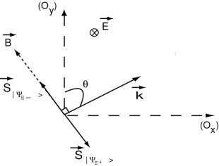
Figure 1: Direction of the virtual magnetic field and spin. An electron with wave vector $\mathbf{k}$ in the presence of an electric field $\mathbf{E}=-E_{0}\;\mathbf{u_{z}}$ feels a virtual field $\mathbf{B}(\mathbf{k},\mathbf{E})$ perpendicular to $\mathbf{k}$.

The spin is aligned or antialigned to this field (see Fig. 1) , so that $\theta(\mathbf{k},\mathbf{S}_{\left|\Psi_{E_{-}}\right>})=\pi/2$, and $\theta(\mathbf{k},\mathbf{S}_{\left|\Psi_{E_{+}}\right>})=-\pi/2$, where $\theta(\mathbf{k},\mathbf{S}_{\left|E_{-}\right>})$ is the angle between $\mathbf{k}$ and the spin $\mathbf{S}$ in the state $\left|\Psi_{E_{-}}\right>$. The amplitude of the magnetic field depends on the velocity of the electron and vanishes for $k=0$, preventing a possible spin polarization in the system. The spin-orbit splitting is usually small compared to the kinetic energy of the electrons ( $0.15$ meV $\leq\alpha k_{f}\leq 1.5$ meV for $E_{f}=14$ meV). Following Ref. LB, , we will introduce a transverse confinement in the leads of the conductor, allowing us to address the longitudinal transport modes for each given transverse mode. Focusing on one lead, $\gamma$, we will make two simplifying assumptions. First, we consider only a single independent transverse mode. Second, we neglect the 1D SO coupling effect that this transverse confining potential could create, since, to our knowledge, there is no experimental verification of this effect, and it is estimated to be much smaller than the Rashba effect MO . Within these approximations, we can use our previous analysis to deduce the eigenstates and the associated energy dispersion diagram (see Fig. 2), with $k$ lying in the direction $x_{\gamma}$ of the lead (making the angle $\theta_{\gamma}$ with the y axis). We will now introduce three labels for the eigenstates that will prove useful in writing the creation and annihilation operators of these states. $\epsilon=a$ or $b$ labels the direction of propagation from the sign of the group velocity $v_{g}$ ($a$ if $sgn(v_{g})>0$, b otherwise). The parameter $k$ labels the longitudinal mode wavevector. The SO coupling label $\sigma\equiv\pm$ designates the two different branches of the energy dispersion diagram for a given k ($+$ branch and $-$ branch in Fig. 2).

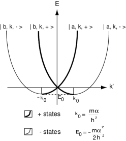
Figure 2: Energy dispersion diagram with SO coupling. The $-\eta_{\sigma}k_{0}\leq k^{\prime}<\infty$ range (a states) is deduced from Eq. (II) with $k^{\prime}=k$. The $-\infty<k^{\prime}<\eta_{\sigma}k_{0}$ range (b states) is then deduced from mirror symmetry ($k^{\prime}=-k$).

Using these labels, we find the following eigenstates and eigenvalues of the system from Eq. (8) and (9)

$$\left|\epsilon,k,\sigma\right> = \Phi(y_{\gamma})\frac{e^{i\eta_{\epsilon}kx_{\gamma}}}{\sqrt{2}}[e^{i\frac{\theta_{\gamma}}{2}}\left|\uparrow\right>+\;\eta_{\epsilon}\eta_{\sigma}e^{-i\frac{\theta_{\gamma}}{2}}\left|\downarrow\right>]$$

$$E = \frac{\hbar k^{2}}{2m}+\eta_{\sigma}\alpha k\;\;\;\;\;-\eta_{\sigma}k_{0}\leq k<\infty$$ (10)

where $\eta_{\epsilon}=+1(-1)$ when $\epsilon=a(b)$, and $\eta_{\sigma}=+1(-1)$ when $\sigma=+(-)$. $\Phi(y_{\gamma})$ is the normalized transverse wavefunction for the transverse mode under consideration. By convention, $k$ is only taken in the range $-\eta_{\sigma}k_{0}\leq k<\infty$ for both the $a$ and $b$ states. We use $\eta_{\epsilon}=\pm 1$ to parameterize explicitly the appropriate wavevector range for the $\epsilon=a(b)$ propagation direction in the eigenstates’ phase factor $e^{i\eta_{\epsilon}kx}$. The eigenvalues in Fig. 2 can be deduced by mirror symmetry. This convention allows us to track the propagation direction throughout the calculation. We also notice in Fig. 2 that, for a given energy, the corresponding $+$ and $-$ states with same label $\epsilon$ do not have the same wavevector:

$$k(E,-)-k(E,+)=\Delta k=2k_{0}=\frac{2m\alpha}{\hbar^{2}}.$$ (11)

The states with $\sigma=\pm$ have their spin perpendicular to the direction of propagation $\mathbf{v_{g}}$ and in opposite directions, so that $\theta(\mathbf{v_{g}},\mathbf{S}_{\left|k,-\right>})=\pi/2$ and $\theta(\mathbf{v_{g}},\mathbf{S}_{\left|k,+\right>})=-\pi/2$ (see Fig. 3).

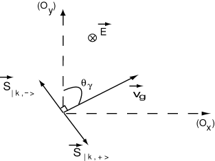
Figure 3: Direction of propagation and direction of the spin

It is important to notice that the $\sigma=+(-)$ states do not coincide with the $\left|\Psi_{E_{+}}\right>\left(\left|\Psi_{E_{-}}\right>\right)$ states, as it is $\mathbf{v_{g}}$, and not $\mathbf{k}$, which determines the direction of the spin (e.g., in Fig. 3, the spin of the $+$ state is perpendicular to and on the right side of $\mathbf{v_{g}}$). For example, in Fig. 2, the two definitions are consistent for states with positive (negative) $k^{\prime}$ and group velocity $v_{g}$. However, they are inconsistent for positive (negative) $k^{\prime}$ and negative (positive) $v_{g}$. We choose here to link the direction of the spin to $\mathbf{v_{g}}$ (rather than $\mathbf{k^{\prime}}$) through the label $\sigma=\pm$ (rather than $E_{\pm}$), because it is the group velocity which determines the direction of the current. Note that in the case without SO coupling, no differentiation between $v_{g}$ and $k^{\prime}$ is necessary since they always share the same sign.

III Spin-Orbit coupling and coherent scattering formalism

The Landauer-Büttiker formalism relies on a second quantization formulation of quantum mechanics. The current is expressed as a function of the field operator, which is expanded in the basis of the scattering states using the operators that create and destroy electrons in the leads of the conductor. A scattering state is a coherent sum of an incident wave in one lead and the outgoing waves it generates in all the other leads. The amplitude of each outgoing wave is given by the scattering matrix $S$, whose elements depend on the properties of the scatterer. As our final goal is to study the fluctuations of the current, it is important to find a simple way to express the time dependence of the current operator. This leads us to choose the stationary states in each lead for the purpose of expanding the field operator. In our rederivation of the coherent scattering formalism, we will follow the same analysis as in Ref. LB, , but introducing two important changes: we will rederive the expression of the current operator as a function of the field operator, adding a new contribution coming from spin-orbit coupling, and we will expand the field operator in the new stationary basis of the SO coupling Hamiltonian.

III.1 Calculation of the current operator

One way to find the current operator for non-interacting electrons is to use the single-particle Schrödinger equation

$$i\hbar\frac{\partial\Psi}{\partial t}=-\frac{\hbar^{2}}{2m}\;(\;\frac{\partial\Psi}{\partial x^{2}}+\frac{\partial\Psi}{\partial y^{2}}\;)+i\alpha\;(\;\sigma_{y}\frac{\partial\Psi}{\partial x}-\sigma_{x}\frac{\partial\Psi}{\partial y}\;),$$ (12)

where $\Psi$ is a two-components spinor. The current operator $\mathbf{\hat{j}}$ can be extracted from the conservation of charge equation $\frac{\partial}{\partial t}[e\Psi^{{\dagger}}\Psi]+\bm{\nabla}.\mathbf{j}=0$; using Eq. (12) and its adjoint,

$$j_{x} = \frac{e\hbar}{2mi}\Big{[}\;\Psi^{{\dagger}}\frac{\partial\Psi}{\partial x}-\frac{\partial\Psi^{{\dagger}}}{\partial x}\Psi\;\Big{]}-\frac{e\alpha}{\hbar}\;\Psi^{{\dagger}}\sigma_{y}\Psi$$ (13)

$$j_{y} = \frac{e\hbar}{2mi}\Big{[}\;\Psi^{{\dagger}}\frac{\partial\Psi}{\partial y}-\frac{\partial\Psi^{{\dagger}}}{\partial y}\Psi\;\Big{]}+\frac{e\alpha}{\hbar}\;\Psi^{{\dagger}}\sigma_{x}\Psi$$ (14)

We can identify the usual kinetic term of the current density

$$\mathbf{j_{K}}=\frac{e\hbar}{2mi}\Big{[}\;\Psi^{{\dagger}}\nabla\Psi-\nabla\Psi^{{\dagger}}\Psi\;\Big{]}.$$ (15)

Note that SO coupling adds a new contribution proportional to $\alpha$ that we call the SO coupling current density $\mathbf{j_{SO}}$,

$$\mathbf{j_{SO}}=-\frac{e\alpha}{\hbar}\;\Psi^{{\dagger}}\sigma_{y}\Psi\;\mathbf{u_{x}}+\frac{e\alpha}{\hbar}\;\Psi^{{\dagger}}\sigma_{x}\Psi\;\mathbf{u_{y}}.$$ (16)

In the framework of second quantization, $\Psi$ becomes a field operator, and we have to expand it using a convenient basis: the stationary states.

III.2 Expansion of the field operator

The first step is to define the creation (annihilation) operators for the SO coupling stationary states. We first introduce the creation operators in the old spin basis: $\hat{a}^{{\dagger}}_{\gamma k\uparrow}$ ($\hat{b}^{{\dagger}}_{\gamma k\downarrow}$) creates an incoming (outgoing) electron with spin up (down) in the first mode of lead $\gamma$ with momentum $k$, in the state $\left|a,k,\uparrow\right>_{\gamma}$ ($\left|b,k,\downarrow\right>_{\gamma}$), where $\left|\epsilon,k,\uparrow\right>_{\gamma}=e^{i\eta_{\epsilon}kx_{\gamma}}\left|\uparrow\right>$. These standard operators satisfy the anticommutation relation $\Big{[}\hat{a}_{\gamma,k,s}\;,\;\hat{a}^{{\dagger}}_{\beta,k^{\prime},s^{\prime}}]_{+}=\delta_{kk^{\prime}}\delta_{\gamma\beta}\delta_{ss^{\prime}}$, where $s$ labels the spin of the electron. Through Eq. (II) we introduce $\hat{a}^{{\dagger}}_{\gamma k\sigma}$, which creates an incoming electron in lead $\gamma$ with momentum $k$ and spin-orbit coupling label $\sigma$ (not to be confused with the spin $s$) satisfying the relation

$$\hat{a}^{{\dagger}}_{\gamma k\sigma}=\frac{1}{\sqrt{2}}[e^{i\frac{\theta_{\gamma}}{2}}\hat{a}^{{\dagger}}_{\gamma k\uparrow}+\eta_{\sigma}e^{-i\frac{\theta_{\gamma}}{2}}\hat{a}^{{\dagger}}_{\gamma k\downarrow}].$$ (17)

Knowing the anticommutation relationships in the spin basis, we can calculate it in our new stationary basis to be

$$\Big{[}\hat{a}_{k,\gamma,\sigma}\;,\;\hat{a}^{{\dagger}}_{k^{\prime},\beta,\sigma^{\prime}}\Big{]}_{+}=\delta_{kk^{\prime}}\delta_{\alpha\beta}\delta_{\sigma\sigma^{\prime}},$$ (18)

where we used the relation $\eta_{\sigma}\eta_{\sigma^{\prime}}=2\delta_{\sigma\sigma^{\prime}}-1$. This result justifies our labeling of the SO coupling eigenstates and the use of the spin-orbit coupling label $\sigma$ instead of the spin. The stationary states form a complete basis, and we can use them to expand the field operator in lead $\gamma$. From now on, we will choose $x_{\gamma}$ and $y_{\gamma}$ as the reference axis (so that $\theta_{\gamma}=\frac{\pi}{2}$), specifically tracking all of the angular dependence in the scattering matrix.

$$\hat{\Psi}(x,y)_{\gamma}=\sum_{\sigma,\epsilon}\sum_{k=-\eta_{\sigma}\;k_{o}}^{\infty}\hat{\epsilon}_{\gamma,k,\sigma}\;\chi^{\epsilon}_{\sigma}\;\frac{e^{i\eta_{\epsilon}kx}\Phi(y)}{\sqrt{L}}$$ (19)

where $\hat{\epsilon}=\hat{a}(\hat{b})$ is the annihilation operator in the incoming(outgoing) states and $\chi^{\epsilon}_{\sigma}$ is a two-component spinor obtained from Eq. (II), setting $\theta_{\gamma}=\frac{\pi}{2}$

$$\left|\epsilon,k,\sigma\right>_{\gamma}=\frac{e^{i\eta_{\epsilon}kx}\;\Phi(y)}{\sqrt{L}}\underbrace{\left[\begin{array}[]{c}\frac{1+i}{2}\\ \eta_{\epsilon}\eta_{\sigma}\frac{1-i}{2}\\ \end{array}\right]}_{\chi^{\epsilon}_{\sigma}}.$$ (20)

As shown in Fig. 4, its spin depends on the SO coupling state ($\sigma$) and on the direction of propagation ($a$ or $b$).

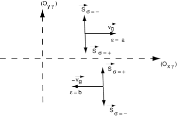
Figure 4: Direction of the spin of $\chi^{\epsilon}_{\sigma}$

At this point, it is more convenient to go from a discrete sum in $k$-space to a continuous integral in energy by defining the operators $\hat{a}^{{\dagger}}(E)$, which create electrons in the energy continuum. As our labeling defines a one-to-one correspondence between ($\epsilon,k,\sigma$) and ($\epsilon,E,\sigma$), we can define unambiguously $\hat{a}^{{\dagger}}_{\gamma\sigma}(E)=\sqrt{\rho(E)}\hat{a}^{{\dagger}}_{\gamma k\sigma}$, so that

$$\Big{[}\hat{a}_{\gamma,\sigma}(E)\;,\;\hat{a}^{{\dagger}}_{\beta,\sigma^{\prime}}(E^{\prime})\Big{]}_{+}=\delta_{\gamma\beta}\delta_{\sigma\sigma^{\prime}}\delta(E-E^{\prime})$$ (21)

where $\rho(E)$ is the density of states at energy E . A priori, $\rho(E)$ could depend on the spin-orbit coupling label $\sigma$, but one can check in Appendix A that it is not the case. Replacing the discrete sum over $k$ by an integral over $E$ and introducing the new operators and their time-dependence $\hat{a}(E,t)=e^{-i\frac{E}{\hbar}t}\hat{a}(E)$, we find

$$\hat{\Psi}(x,y,t)_{\gamma}=\frac{1}{\sqrt{2\pi}}\sum_{\sigma,\epsilon}\int_{E_{0}}^{\infty}\frac{dE}{\sqrt{\hbar\;v_{g}(E)}}\hat{\epsilon}_{\gamma,\sigma}(E)\;\chi^{\epsilon}_{\sigma}\Phi(y)$$

$$\times\;e^{i\eta_{\epsilon}k(E,\sigma)x}e^{-i\frac{E}{\hbar}t}\qquad$$ (22)

with $E_{0}\equiv-\frac{m\alpha^{2}}{2\hbar^{2}}$, and $k$ has been replaced by $k(E,\sigma)$ to remind us that, for a given energy, $k$ depends on the spin-orbit coupling label $\sigma$.

III.3 Current in the spin-orbit coupling basis

The current in lead $\gamma$ is given by

$$\hat{I}_{\alpha}=\int dy\hat{j}_{x}=\int dy(\hat{j}_{xK}+\hat{j}_{xSO})\equiv\hat{I}_{K}+\hat{I}_{SO}.$$ (23)

We will begin by calculating the usual kinetic term $\hat{I}_{K}$. Using Eq. (15), we have

$$\hat{I}_{K}(t)=\sum_{\sigma\sigma^{\prime}}\sum_{\epsilon\;\epsilon^{\prime}}\int dEdE^{\prime}\;\hat{I}_{K\;\sigma\sigma^{\prime}}^{\;\epsilon\;\epsilon^{\prime}}(E,E^{\prime})\;\hat{\epsilon}^{+}_{\gamma\sigma}(E)\;\hat{\epsilon^{\prime}}_{\gamma\sigma^{\prime}}(E^{\prime})\;e^{i\frac{E-E^{\prime}}{\hbar}t}.$$ (24)

$$\hat{I}_{K\;\sigma\sigma^{\prime}}^{\;\epsilon\;\epsilon^{\prime}}(E,E^{\prime})\;=\;\frac{e\hbar}{2mi}\;\frac{i\chi_{\sigma}^{\epsilon^{{\dagger}}}\chi_{\sigma^{\prime}}^{\epsilon^{\prime}}}{h\sqrt{v_{g}(E)v_{g}(E^{\prime})}}[\;\eta_{\epsilon}k(E,\sigma)+\eta_{\epsilon^{\prime}}k(E^{\prime},\sigma^{\prime})\;]\;e^{i\;(\eta_{\epsilon^{\prime}}k(E^{\prime},\sigma^{\prime})-\eta_{\epsilon}k(E,\sigma))x}.$$ (25)

We notice from Eq. (24) that the $\omega$ frequency of the current is given by $E=E^{\prime}+\hbar\omega$. Following Ref. LB, , we calculate the current and noise in the zero-frequency limit, and make the approximation $k(E^{\prime},\sigma)\approx k(E,\sigma)$ (as $E\approx E^{\prime}$) for electrons having the same SO coupling label, and, using Eq. (11), $k(E^{\prime},\sigma^{\prime})=k(E,\sigma)+\eta_{\sigma}\Delta k$ for electrons having different SO coupling labels. From Eq. (20), we also have, (with $\delta_{\epsilon\neq\epsilon^{\prime}}=1$ if $\epsilon\neq\epsilon^{\prime},0$ otherwise)

$$\chi_{\sigma}^{\epsilon^{{\dagger}}}\chi_{\sigma^{\prime}}^{\epsilon^{\prime}}=\delta_{\epsilon\epsilon^{\prime}}\delta_{\sigma\sigma^{\prime}}+\delta_{\epsilon\neq\epsilon^{\prime}}\delta_{\sigma\neq\sigma^{\prime}}.$$ (26)

This result is consistent with the fact that only electrons with the same direction of propagation and the same spin-orbit coupling label, or opposite direction of propagation and opposite spin-orbit coupling label, have the same spin.

In the $\sigma=\sigma^{\prime}$ case, implying $\epsilon=\epsilon^{\prime}$ and $k(E^{\prime},\sigma^{\prime})\approx k(E,\sigma)$, we find

$$\hat{I}_{K\;\sigma\sigma^{\prime}}^{\;\epsilon\;\epsilon^{\prime}}(E,E^{\prime})\mid_{\sigma=\sigma^{\prime}}\;=\;\eta_{\epsilon}\frac{e}{h}\;\frac{k(E,\sigma)}{k(E,+)+\frac{m\alpha}{\hbar^{2}}}.$$ (27)

In the $\sigma\neq\sigma^{\prime}$ case, implying $\epsilon\neq\epsilon^{\prime}$ and $k(E^{\prime},\sigma^{\prime})\approx k(E,\sigma)+\eta_{\sigma}\frac{2m\alpha}{\hbar^{2}}$, so that $\eta_{\epsilon}k(E,\sigma)+\eta_{\epsilon^{\prime}}k^{\prime}(E,\sigma^{\prime})=-\eta_{\epsilon}\;\eta_{\sigma}\frac{2m\alpha}{\hbar^{2}}$, we find

$$\hat{I}_{K\;\sigma\sigma^{\prime}}^{\;\epsilon\;\epsilon^{\prime}}(E,E^{\prime})\mid_{\sigma\neq\sigma^{\prime}}\;=\;-\eta_{\epsilon}\frac{e}{h}\;\frac{\eta_{\sigma}\frac{m\alpha}{\hbar^{2}}}{k(E,+)+\frac{m\alpha}{\hbar^{2}}}\;e^{-i\eta_{\epsilon}(2k(E,\sigma)+\eta_{\sigma}\Delta k)x}.$$ (28)

If we only consider the kinetic term of the current, a non-vanishing contribution for $\epsilon\neq\epsilon^{\prime}$ leads to terms like $\hat{a}^{{\dagger}}\hat{b}$ and $\hat{b}^{{\dagger}}\hat{a}$ in the expression of the current, corresponding to electrons propagating in opposite directions.

Now, let us study the contribution of the spin-orbit coupling current $\hat{I}_{SO}$. Using Eq. (16) to calculate $\hat{I}^{\;\epsilon\;\epsilon^{\prime}}_{SO\;\sigma\sigma^{\prime}}$ in Eq. (24) with $\scriptstyle K\rightarrow SO$, we find

$$\hat{I}^{\;\epsilon\;\epsilon^{\prime}}_{SO\;\sigma\sigma^{\prime}}(E,E^{\prime})=-\frac{e}{h}\;\frac{\frac{\alpha}{\hbar}}{\sqrt{v_{g}(E)v_{g}(E^{\prime})}}\;\chi_{\sigma}^{\epsilon^{{\dagger}}}\sigma_{y}\chi_{\sigma^{\prime}}^{\epsilon^{\prime}}\;e^{i(\eta_{\epsilon^{\prime}}k(E^{\prime},\sigma^{\prime})-\eta_{\epsilon}k(E,\sigma))x}.$$ (29)

Using $\eta_{\epsilon^{\prime}}\eta_{\sigma^{\prime}}=\eta_{\epsilon}\eta_{\sigma}$, we have from Eq. (20) $\sigma_{y}\chi_{\sigma^{\prime}}^{\epsilon^{\prime}}=-\eta_{\epsilon^{\prime}}\eta_{\sigma^{\prime}}\chi_{\sigma^{\prime}}^{\epsilon^{\prime}}$ and $\chi_{\sigma}^{\epsilon^{{\dagger}}}\sigma_{y}\chi_{\sigma^{\prime}}^{\epsilon^{\prime}}=-\eta_{\epsilon}\eta_{\sigma}\;(\delta_{\epsilon\epsilon^{\prime}}\;\delta_{\sigma\sigma^{\prime}}\;+\;\delta_{\epsilon\neq\epsilon^{\prime}}\;\delta_{\sigma\neq\sigma^{\prime}})$, so that

$$\hat{I}^{\;\epsilon\;\epsilon^{\prime}}_{SO\;\sigma\sigma^{\prime}}(E,E^{\prime})=\eta_{\epsilon}\frac{e}{h}\;\frac{\eta_{\sigma}\;\frac{m\alpha}{\hbar^{2}}}{k(E,+)+\frac{m\alpha}{\hbar^{2}}}\;\Big{[}\;\delta_{\epsilon\epsilon^{\prime}}\;\delta_{\sigma\sigma^{\prime}}+\;e^{-i\eta_{\epsilon}(2k(E,\sigma)+\eta_{\sigma}\Delta k)x}\;\delta_{\epsilon\neq\epsilon^{\prime}}\;\delta_{\sigma\neq\sigma^{\prime}}\;\Big{]}.$$ (30)

We can now calculate the value of the total current from Eq. (27), (28) and (30)

$$\hat{I}^{\;\epsilon\;\epsilon^{\prime}}_{\;\sigma\sigma^{\prime}}(E,E^{\prime}) = \hat{I}^{\;\epsilon\;\epsilon^{\prime}}_{K\;\sigma\sigma^{\prime}}(E,E^{\prime})+\hat{I}^{\;\epsilon\;\epsilon^{\prime}}_{SO\;\sigma\sigma^{\prime}}(E,E^{\prime})$$ (31)

$$= \eta_{\epsilon}\frac{e}{h}\;\delta_{\epsilon\epsilon^{\prime}}\;\delta_{\sigma\sigma^{\prime}}.$$

Although the spin-orbit coupling mixes electrons having different directions of propagation when we consider only the kinetic term of the current, these contributions cancel when we add the spin-orbit coupling current $I_{SO}$, and we find the standard formula for the current operator,

$$\hat{I}\;=\;\frac{e}{h}\sum_{\sigma}\int dE\;dE^{\prime}\;[\;\hat{a}^{{\dagger}}_{\gamma\sigma}(E)\;\hat{a}_{\gamma\sigma}(E^{\prime})\qquad$$

$$-\hat{b}^{{\dagger}}_{\gamma\sigma}(E)\;\hat{b}_{\gamma\sigma}(E^{\prime})\;]\;e^{i\frac{E-E^{\prime}}{\hbar}t}.$$ (32)

In this formula, the definition of the $\hat{a}$($\hat{b}$) states as states with positive(negative) group velocity, and not necessarily positive(negative) wavevector, is consistent with the fact that they carry the current in opposite directions. More importantly, the final expression of the current is similar to the one found in Ref. LB, , but with the spin index replaced by the spin-orbit coupling label $\sigma=\pm$. The spin related to this new index depends on the direction of propagation, that is, the angle of the lead $\theta_{\gamma}$. Therefore, we expect a $\theta_{\gamma}$ dependence in the scattering matrix relating the spin-orbit coupling states in leads with different orientations. As an example, we investigate the scattering matrix in the case of a four-port beamsplitter (two input leads, two output leads) used in electron collisions. The scattering matrix relates the outgoing states in the outputs ($\hat{b}$ states) to the incident states at the input ($\hat{a}$ states)

$$\hat{b}_{\gamma\sigma}=\sum_{\beta\sigma^{\prime}}S^{\gamma\sigma}_{\beta\sigma^{\prime}}\;\hat{a}_{\beta\sigma^{\prime}}.$$ (33)

In the spin-independent transport case, as the beamsplitter does not act on the spin degrees of freedom, the scattering matrix does not mix different spins (the scattering matrix is diagonal in each subspace of spin: spin-up and spin-down). In this case the reflection and transmission coefficients do not depend on the spin. However, when we include spin-orbit coupling, the situation is more complicated, because the spin associated with the spin-orbit coupling label $\sigma$ is different in each lead (the leads having different orientations). The conservation of the spin at the beamsplitter then implies that we have a mixing of the spin-orbit states (off-diagonal elements in the scattering matrix), and this mixing becomes more important when the angle between the leads increases.

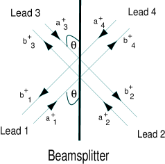
Figure 5: Four-port beamsplitter

A beamsplitter, with all leads oriented at the same angle $\theta$ (the case illustrated in Fig. 5) is investigated in Appendix B, and the following scattering matrix is found after some simplifying assumptions

$$\left(\begin{array}[]{c}\hat{b}_{3+}\\ \hat{b}_{3-}\\ \hat{b}_{4+}\\ \hat{b}_{4-}\end{array}\right)=\underbrace{\left(\begin{array}[]{cccc}r\cos\theta&i\;r\sin\theta&t&0\\ i\;r\sin\theta&r\cos\theta&0&t\\ t&0&r\cos\theta&-i\;r\sin\theta\\ 0&t&-i\;r\sin\theta&r\cos\theta\end{array}\right)}_{S}\left(\begin{array}[]{c}\hat{a}_{1+}\\ \hat{a}_{1-}\\ \hat{a}_{2+}\\ \hat{a}_{2-}\end{array}\right)$$ (46)

We note that the unitarity of the $S$ matrix requires $\left|r\right|^{2}+\left|t\right|^{2}\equiv R+T=1$ and $rt^{*}+tr^{*}=0$.

IV Spin-orbit coupling and noise in electron collisions

We will now use the expression of the current operator and the scattering matrix to calculate the current and noise in two experiments using the four-port beamsplitter setup. The first is an unpolarized electron collision, which has already been realized experimentally (see Ref. EC, ). The second is a spin-polarized electron collision.

IV.1 Unpolarized electron collision

This experiment is a collision at a 50/50 beamsplitter of electrons from leads 1 and 2 which are biased at $E_{f}+eV.$ At zero temperature and without spin-orbit coupling, each electron with a specific spin in lead 1 has an identical partner in lead 2. The Pauli exclusion principle then forbids us to find these two electrons in the same output. We expect a total suppression of the partition noise. With spin-orbit coupling, we do not expect this result to be modified. It relies only on the full occupation of the energy eigenstates, which is not modified at zero temperature by SO coupling. We will confirm this by studying the collision of four electrons at the same energy. The initial state is:

$$\left|\Psi_{i}\right>=\hat{a}^{{\dagger}}_{k,+,1}(E)\;\hat{a}^{{\dagger}}_{k^{\prime},-,1}(E)\;\hat{a}^{{\dagger}}_{k,+,2}(E)\;\hat{a}^{{\dagger}}_{k^{\prime},-,2}(E)\;\left|0\right>,$$ (47)

From now on, we will drop the $E$, $k$ and $k^{\prime}$ labels for the energy and the momentum of the electrons, associating a $+$($-$) SO coupling state with $k$($k^{\prime}$). The output state is found using the new scattering matrix with SO coupling using Eq. (33) and Eq. (46)

$$\left|\Psi_{f}\right> = \left[r\;[\;\cos\theta\;\hat{b}^{{\dagger}}_{+3}+i\sin\theta\;\hat{b}^{{\dagger}}_{-3}\;]+t\;\hat{b}^{{\dagger}}_{+4}\right]\;\left[r\;[\;i\sin\theta\;\hat{b}^{{\dagger}}_{+3}+\cos\theta\;\hat{b}^{{\dagger}}_{-3}\;]+t\;\hat{b}^{{\dagger}}_{-4}\right]$$ (48)

$$\times\left[t\;\hat{b}^{{\dagger}}_{+3}+r\;[\;\cos\theta\;\hat{b}^{{\dagger}}_{+4}-i\sin\theta\;\hat{b}^{{\dagger}}_{-4}\;]\right]\;\left[t\;\hat{b}^{{\dagger}}_{-3}+r\;[\;-i\sin\theta\;\hat{b}^{{\dagger}}_{+4}+\cos\theta\;\hat{b}^{{\dagger}}_{-4}\;]\right]\left|0\right>$$

$$= \hat{b}^{{\dagger}}_{+3}\hat{b}^{{\dagger}}_{-3}\hat{b}^{{\dagger}}_{+4}\hat{b}^{{\dagger}}_{-4}\left|0\right>$$

where we have used the relation $r^{4}+t^{4}-2\;r^{2}\;t^{2}=1$. As expected, a full occupation of the two input states at energy E leads to a full occupation of the two output states as well. A calculation of the noise for the fully occupied outputs would show a complete suppression of the partition noise. The only difference with the spin-independent transport case is that the colliding electrons at the same energy do not have the same momentum ($k\neq k^{\prime}$). Therefore, the non-ideality in the noise suppression observed in Ref. EC, cannot be caused by the SO coupling.

IV.2 Spin-polarized electron collision

In the previous example, an unpolarized collision cannot show any SO coupling effect, because, starting with two quiet sources of electrons with fully occupied energy levels, all the transport statistics are governed by the Pauli exclusion principle independent of the SO coupling. However, this is not the case for a spin-polarized collision. As the standard spin basis is not the stationary basis, and as the SO coupling scattering matrix mixes different SO coupling states, some of the partition noise is recovered, depending on the SO coupling constant $\alpha$ and on the angle between the colliding leads. We will confirm this by calculating the non-equilibrium noise (of the electrons above the Fermi sea) between $E_{f}$ and $E_{f}+eV$, assuming that the process of polarization does not effect the transport in the conductor (for example, there is no magnetic field in the conductor). The input state is then made of all the electrons with the same spin, for example spin-up, between $k_{f}$ and $k_{\max}=k(E_{f}+eV)$. Following Ref. LB, , we present the initial state and the current operator using the following notations

$$\left|\Psi_{i}\right> = \prod_{k=k_{f}}^{k_{max}}\hat{a}^{{\dagger}}_{1\uparrow}(k)\hat{a}^{{\dagger}}_{2\uparrow}(k)\left|0\right>$$ (49)

$$\hat{I}_{\alpha}(t) = \frac{e}{h}\sum_{s}\sum_{\sigma\sigma^{\prime}}\sum_{\beta\gamma}\int dEdE^{\prime}e^{\frac{i(E-E^{\prime})t}{\hbar}}A^{\alpha s}_{\beta\gamma\sigma\sigma^{\prime}}$$ (50)

$$\qquad\qquad\qquad\quad\times\;\hat{a}^{{\dagger}}_{\beta\sigma}(E)\hat{a}_{\gamma\sigma^{\prime}}(E^{\prime})$$

$$A^{\alpha s}_{\beta\gamma\sigma\sigma^{\prime}} = \delta_{\alpha\beta}\delta_{\alpha\gamma}\delta_{s\sigma}\delta_{s\sigma^{\prime}}-S^{*\alpha s}_{\beta\sigma}S^{\alpha s}_{\gamma\sigma^{\prime}}$$ (51)

where $k_{max}$ is given by $E_{f}+eV=\frac{\hbar^{2}k_{max}^{2}}{2m}$. We then use the current fluctuation $\delta\hat{I}_{\alpha}(t)=\hat{I}_{\alpha}(t)-\left<\hat{I}_{\alpha}(t)\right>$ to calculate the fluctuation correlation function.

$$\left<\delta\hat{I}_{\alpha}(t)\delta\hat{I}_{\alpha}(0)\right> = \frac{e^{2}}{h^{2}}\sum_{ss^{\prime}}\sum_{\sigma\sigma^{\prime}\sigma^{\prime\prime}\sigma^{\prime\prime\prime}}\sum_{\beta\gamma\delta\zeta}\int dEdE^{\prime}dE^{\prime\prime}dE^{\prime\prime\prime}e^{\frac{i(E-E^{\prime})t}{\hbar}}A^{\alpha s}_{\beta\gamma\sigma\sigma^{\prime}}A^{\alpha s^{\prime}}_{\delta\zeta\sigma^{\prime\prime}\sigma^{\prime\prime\prime}}\;\Delta^{\sigma\sigma^{\prime}\sigma^{\prime\prime}\sigma^{\prime\prime\prime}}_{\beta\gamma\delta\zeta}$$ (52)

$$\Delta^{\sigma\sigma^{\prime}\sigma^{\prime\prime}\sigma^{\prime\prime\prime}}_{\beta\gamma\delta\zeta} \equiv \left<\hat{a}^{{\dagger}}_{\beta\sigma}(E)\hat{a}_{\gamma\sigma^{\prime}}(E^{\prime})\hat{a}^{{\dagger}}_{\delta\sigma^{\prime\prime}}(E^{\prime\prime})\hat{a}_{\zeta\sigma^{\prime\prime\prime}}(E^{\prime\prime\prime})\right>-\left<\hat{a}^{{\dagger}}_{\beta\sigma}(E)\hat{a}_{\gamma\sigma^{\prime}}(E^{\prime})\right>\left<\hat{a}^{{\dagger}}_{\delta\sigma^{\prime\prime}}(E^{\prime\prime})\hat{a}_{\zeta\sigma^{\prime\prime\prime}}(E^{\prime\prime\prime})\right>$$ (53)

Although we derived an expression for the current operator in the SO coupling basis, it is mathematically more convenient in this case to express all the operators in the standard spin basis

$$\hat{a}^{{\dagger}}_{\beta\sigma}(E)=\frac{[\;e^{i\frac{\theta_{\beta}}{2}}\hat{a}^{{\dagger}}_{\beta\uparrow}(k(E,\sigma))+\eta_{\sigma}e^{-i\frac{\theta_{\beta}}{2}}\hat{a}^{{\dagger}}_{\beta\downarrow}(k(E,\sigma))\;]}{\sqrt{2D_{\sigma}(k)}}$$ (54)

with $D_{\sigma}(k)\equiv\frac{dE(k,\sigma)}{dk}=\frac{\hbar^{2}k}{m}+\eta_{\sigma}\alpha$. Defining $\Pi\equiv\sqrt{D_{\sigma}(k)D_{\sigma^{\prime}}(k^{\prime})D_{\sigma^{\prime\prime}}(k^{\prime\prime})D_{\sigma^{\prime\prime\prime}}(k^{\prime\prime\prime})}$, we have,

$$\Delta^{\sigma\sigma^{\prime}\sigma^{\prime\prime}\sigma^{\prime\prime\prime}}_{\beta\gamma\delta\zeta} = \frac{1}{4\Pi}\;\Big{[}\;\delta_{\beta\zeta}\delta_{\gamma\delta}\;\delta(k_{E,\sigma}-k_{E^{\prime\prime\prime},\sigma^{\prime\prime\prime}})\;\delta(k_{E^{\prime},\sigma^{\prime}}-k_{E^{\prime\prime},\sigma^{\prime\prime}})\;n_{\beta\uparrow}(k_{E,\sigma})\;[1-n_{\gamma\uparrow}(k_{E^{\prime},\sigma^{\prime}})]\;$$ (55)

$$\!\!\!\!\!\!\qquad\qquad...+\;\eta_{\sigma^{\prime}}\eta_{\sigma^{\prime\prime}}\delta_{\beta\zeta}\delta_{\gamma\delta}\;\delta(k_{E,\sigma}-k_{E^{\prime\prime\prime},\sigma^{\prime\prime\prime}})\delta(k_{E^{\prime},\sigma^{\prime}}-k_{E^{\prime\prime},\sigma^{\prime\prime}})\;n_{\beta\uparrow}(k_{E,\sigma})\;\Big{]}$$

where $k_{E,\sigma}=k_{E^{\prime},\sigma^{\prime}}$ for $E=E^{\prime}+\alpha k(\eta_{\sigma^{\prime}}-\eta_{\sigma})$, so that $\delta(k_{E,\sigma}-k_{E^{\prime\prime\prime},\sigma^{\prime\prime\prime}})=D_{\sigma}(k)\delta[E-E^{\prime\prime\prime}+\alpha k(\eta_{\sigma}-\eta_{\sigma^{\prime\prime\prime}})]$. After integration over $E^{{}^{\prime\prime}}$ and $E^{{}^{\prime\prime\prime}}$ and making the approximation $D_{+}(k)\approx D_{-}(k)$, we find

$$\int dE^{\prime\prime}dE^{\prime\prime\prime}\Delta^{\sigma\sigma^{\prime}\sigma^{\prime\prime}\sigma^{\prime\prime\prime}}_{\beta\gamma\delta\zeta} = \frac{1}{4}\Big{[}\;\delta_{\beta\zeta}\delta_{\gamma\delta}\;n_{\beta\uparrow}(k_{E,\sigma})\;[1-n_{\gamma\uparrow}(k_{E^{\prime},\sigma^{\prime}})]\;+\;\eta_{\sigma^{\prime}}\eta_{\sigma^{\prime\prime}}\;\delta_{\gamma\delta}\;n_{\beta\uparrow}(k_{E,\sigma})\;\Big{]}.$$ (56)

We can replace $D_{-}(k)$ by $D_{+}(k)$, because $\frac{D_{-}(k)}{D_{+}(k)}=\frac{\frac{\hbar^{2}k}{m}-\alpha}{\frac{\hbar^{2}k}{m}+\alpha}\approx 1+\frac{\alpha}{\frac{\hbar^{2}k}{2m}}\approx 1$, which follows from $\frac{\alpha}{\frac{\hbar^{2}k}{2m}}\leq\frac{\alpha k_{f}}{\frac{\hbar^{2}k_{f}^{2}}{2m}}=\frac{E_{SO}(k_{f})}{E_{c}(k_{f})}\ll 1$ as the SO coupling is small. We will now calculate the power spectral density at zero frequency in output lead number 3, $S_{33}(0)$,

$$S_{33}(\omega)\equiv 2\;\int dt\;e^{i\omega t}\left<\delta I_{3}(t)\;\delta I_{3}(0)\right>.$$ (57)

From Eq. (52) and Eq. (56), we find

$$S_{33}(0)=\frac{e^{2}}{2h}\sum_{ss^{\prime}}\sum_{\sigma\sigma^{\prime}\sigma^{\prime\prime}\sigma^{\prime\prime\prime}}\sum_{\beta,\gamma=1,2}A^{3s}_{\beta\gamma\sigma\sigma^{\prime}}\;A^{3s^{\prime}}_{\gamma\beta\sigma^{\prime\prime}\sigma^{\prime\prime\prime}}$$

$$\times\int dE\;n_{\beta\uparrow}(k_{E,\sigma})[1-n_{\gamma\uparrow}(k_{E,\sigma^{\prime}})+\eta_{\sigma^{\prime}}\eta_{\sigma^{\prime\prime}}]$$ (58)

where $\gamma=$ 1 or 2, since we ignored scattering from output to output. $n_{\beta\uparrow}(k_{E,\sigma})$ is the number of electrons in lead $\beta$ with spin up and momentum $k_{E,\sigma}$

$$\begin{array}[]{l}n_{\beta\uparrow}(k_{E,\sigma})=\\ \\ \;\left\{\begin{array}[]{l}0\;\;\text{ if }\;\;E\leq E_{f}+\eta_{\sigma}\alpha k_{f}\\ 1\;\;\text{if}\;\;E_{f}+\eta_{\sigma}\alpha k_{f}\leq E\leq E_{f}+eV+\eta_{\sigma}\alpha k_{max}\\ 0\;\;\text{if}\;\;E_{f}+eV+\eta_{\sigma}\alpha k_{max}\leq E\end{array}\right..\\ \end{array}$$

Assuming that the SO coupling is weaker than the bias voltage, that is, $E_{f}+\alpha k_{f}\leq E_{f}+eV-\alpha k_{max}$, we have $n_{\beta\uparrow}(k_{E,-})[1-n_{\gamma\uparrow}(k_{E,+})]\neq 0$ for $E_{f}-\alpha k_{f}\leq E\leq E_{f}+\alpha k_{f}$ and $n_{\beta\uparrow}(k_{E,+})[1-n_{\gamma\uparrow}(k_{E,-})]\neq 0$ for $E_{f}+eV-\alpha k_{max}\leq E\leq E_{f}+eV-\alpha k_{max}$. Therefore, Eq. (58) becomes

$$S_{33}(0)=\frac{e^{2}}{2h}\sum_{ss^{\prime}}\sum_{\sigma\sigma^{\prime}\sigma^{\prime\prime}\sigma^{\prime\prime\prime}}\sum_{\beta,\gamma}A^{3s}_{\beta\gamma\sigma\sigma^{\prime}}\;A^{3s^{\prime}}_{\gamma\beta\sigma^{\prime\prime}\sigma^{\prime\prime\prime}}[\;\eta_{\sigma^{\prime}}\eta_{\sigma^{\prime\prime}}\;eV+\delta_{\sigma+}\delta_{\sigma^{\prime}-}\;2\;\alpha k_{max}+\delta_{\sigma-}\delta_{\sigma^{\prime}+}\;2\;\alpha k_{f}].$$ (59)

Given the scattering matrix calculated in Eq. (46), we find

$$\sum_{ss^{\prime}}\sum_{\sigma\sigma^{\prime}\sigma^{\prime\prime}\sigma^{\prime\prime\prime}}\sum_{\beta,\gamma}A^{3s}_{\beta\gamma\sigma\sigma^{\prime}}\;A^{3s^{\prime}}_{\gamma\beta\sigma^{\prime\prime}\sigma^{\prime\prime\prime}}\eta_{\sigma^{\prime}}\eta_{\sigma^{\prime\prime}}=0,$$ (60)

and

$$\sum_{ss^{\prime}}\sum_{\sigma\sigma^{\prime}\sigma^{\prime\prime}\sigma^{\prime\prime\prime}}\sum_{\beta,\gamma}A^{3s}_{\beta\gamma\sigma\sigma^{\prime}}\;A^{3s^{\prime}}_{\gamma\beta\sigma^{\prime\prime}\sigma^{\prime\prime\prime}}\delta_{\sigma+}\delta_{\sigma^{\prime}-}=4\;TR\sin^{2}\theta,$$ (61)

so that

$$S_{33}(0)=\frac{4e^{2}}{h}\;(\alpha k_{f}+\alpha k_{max})\;T(1-T)\sin^{2}\theta.$$ (62)

After some calculation, we find the current and Fano factor to be

$$\left<I_{3}\right> = \frac{e^{2}V}{h}$$ (63)

$$F \equiv \frac{S_{33}(0)}{\left<I_{3}\right>}\;=\;4\;eT(1-T)\sin^{2}\theta\;\frac{\alpha(k_{f}+k_{max})}{eV}.$$

This result reveals two typical features of SO coupling: first, the noise is proportional to the SO coupling constant, and second, it depends on the angle between the input leads 1 and 2. One can check that the obtained noise is identical to the partition noise for two independent leads where only a fraction ($\frac{\alpha(k_{f}+k_{max})}{eV})$ of the electrons is colliding, and for which the noise is modified by the factor $\sin^{2}\theta$.

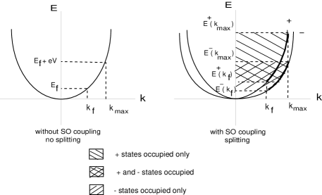
Figure 6: Energy diagrams with and without SO coupling

This result can also be explained using Fig. 6. In the inputs, the spin-up electron states between $k_{f}$ and $k_{max}$ are fully occupied. However, in terms of the SO coupling states, only the states between $E(k_{f},+)$ and $E(k_{max},-)$ are jointly occupied, giving no contribution to the noise as in the unpolarized case. Between $E(k_{f},-)$ and $E(k_{f},+)$, only the $-$ states are filled, and between $E(k_{max},-)$ and $E(k_{max},+)$, only the $+$ states are filled. These states do not have the same spin in leads 1 and 2 (their overlap is $\cos^{2}\theta$), so that the Pauli exclusion principle does not fully suppress the noise, and the classical partition noise is partially recovered through the factor $\sin^{2}\theta=1-\cos^{2}\theta$. In this treatment, we have assumed that the SO coupling is small ($\frac{\alpha(k_{f}+k_{max})}{eV}\leq 1$), so that $E(k_{f},+)\leq E(k_{max},-)$. But, a typical value of the applied bias voltage is $eV=0.1$ meV, which is smaller than the typical values of energy splitting caused by the Rashba effect ($0.3$ meV $\leq 2\alpha k_{f}\leq 3$ meV). In this case, all the electrons contribute to the partition noise, and we have $F=4\;eT(1-T)\sin^{2}\theta$. Depending on the angle between the leads, we can go from full noise suppression to the classical limit of the partition noise. The modification of the noise caused by SO coupling in this collision experiment can in principle be measured, even for small values of the SO coupling constant.

V Conclusion

We have studied the influence of SO coupling in the framework of the Landauer-Büttiker formalism. A short review of the effect of SO coupling in 2DEGs (and more precisely of the Rashba effect) has reminded us of its main features: spin-splitting proportional to $k$, and stationary states of the spin perpendicular to the direction of propagation. The electron feels a magnetic field perpendicular to the direction of propagation, with an amplitude proportional to the velocity. We have then included the effects of SO coupling in the Landauer-Büttiker coherent scattering formalism. The SO coupling gave rise to two important modifications. First, the addition of a SO coupling term in the Hamiltonian modifies the expression of the current operator, and an extra term directly related to SO coupling has to be included. Second, the expansion of the current operator is in the basis of the stationary states of SO coupling. The final formula for the current operator was found to be identical to the one derived in the spin-independent transport case, but with the spin replaced by the SO coupling label, indicating the alignment of the spin on the virtual magnetic field caused by the SO coupling. The main differences introduced by the SO coupling then arise in the calculation of the scattering matrix relating the stationary states of SO coupling in different leads with different orientations. The direction of the virtual magnetic field (and, consequently, the direction of the spin) depends on the direction of propagation which is different for each lead in general. Therefore, the scattering matrix is shown to mix states with different SO coupling labels, and the strength of this mixing depends on the angle between the leads. The effect of SO coupling on the current noise was then investigated in two examples of electron collision. In the unpolarized electron collision example, it is shown that the SO coupling does not modify the noise; this case is entirely determined by the Pauli exclusion principle. In contrast, the polarized case exhibits a contribution to the noise caused by SO coupling, which is proportional to the SO coupling constant $\alpha$ and depends on the angle between the leads. A polarized electron collision experiment provides, in principle, another way to measure the strength of the Rashba splitting energy. Finally, this new formulation of the current operator can be applied to other coherent scattering experiments in which one wants to investigate or incorporate the effects of SO coupling.

Appendix A Density of states with spin-orbit coupling

In this appendix, we calculate the density of states and show that it does not depend on the SO coupling label $\sigma$, as is suggested by the symmetry between the $+$ and $-$ states in the energy dispersion diagram (see Fig. 2),

$$E = \frac{\hbar^{2}k^{2}(E,\sigma)}{2m}+\eta_{\sigma}\alpha k(E,\sigma)$$ (65)

$$v_{g\sigma}(E) = \frac{1}{\hbar}\frac{dE(k,\sigma)}{dk}\;=\;\frac{\hbar\;k(E,\sigma)}{m}+\eta_{\sigma}\frac{\alpha}{\hbar}.$$ (66)

From Eq. (11) we deduce

$$k(E,\sigma) = k(E,+)+(\eta_{\sigma}-1)\frac{m\alpha}{\hbar^{2}}$$ (67)

$$v_{g\sigma}(E) = \frac{\hbar k(E,+)}{m}+\frac{\alpha}{\hbar}\;=\;v_{g}(E)$$ (68)

$$\rho(E) = \frac{\rho(k)}{\hbar\;v_{g}(E)}\;=\;\frac{L}{2\pi}\frac{1}{\hbar\;v_{g}(E)}$$ (69)

which is independent of $\sigma$.

Appendix B Scattering matrix in the four-port beamsplitter case

Here, we determine the scattering matrix for the four-port beamsplitter described in Fig. 5. The beamsplitter is very simply approximated by a potential barrier at $V=V_{0}$ of length $L$. The plane is then divided into three areas of different potential (see Fig. 7) in which the solution of the Schrödinger equation is known.

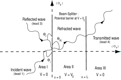
Figure 7: Reflected, refracted and transmitted waves in a beamsplitter

Starting with an incident wave in lead number one, for example, we can calculate the reflected, refracted, and transmitted waves in lead 3 and 4, using the continuity of the wavefunction and its derivatives at the beamsplitter interface (x=0 and x=$L$). For example, let us start with an incident state at energy $E$ with momentum $k_{i}$ in the SO coupling state $\sigma=+$. By the conservation of energy, the reflected wave in lead 3 is a superposition of the states $\left|\mathbf{k_{r}}(E,+),+\right>$ and $\left|\mathbf{k_{r}}(E,-),-\right>$ with

$$k_{r}(E,+)=k_{i}(E,+)=k_{r}(E,-)-\Delta k.$$ (70)

The translational invariance of the beamsplitter along the y-axis leads to the conservation of the y-component of the momentum

$$k_{i}\cos\theta_{i}=k_{r}(E,+)\cos\theta_{+}=k_{r}(E,-)\cos\theta_{-}.$$ (71)

We deduce that $\cos\theta_{i}=\cos\theta_{r+}$, but $\cos\theta_{i}\neq\cos\theta_{r-}$. There is dispersion due to the SO coupling, leading to an angular separation between the $+$ and $-$ states after reflection at the beamsplitter (see Fig. 8).

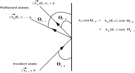
Figure 8: angular separation after reflection at a beamsplitter

This angular separation is given by

$$\theta_{r-}=\arccos[(1-\frac{\Delta k}{k_{r}(E,-)})\cos\theta_{i}]\neq\theta_{r+}.$$ (72)

Starting with an incident state with SO coupling label $-$, the angular separation is

$$\theta_{r+}=\arccos[(1+\frac{\Delta k}{k_{r}(E,+)})\cos\theta_{i}]\neq\theta_{r-}.$$ (73)

In analogy with the the total reflection for incident angles below the critical angle in classical optics, we can even have $(1+\frac{\Delta k}{k_{r}(E,+)})\cos\theta_{i}>1$, leading to a suppression of the reflection in the $+$ state for a small enough incident angle. We note that starting with a mixture of $+$ and $-$ states in the incident beam of electrons, one could suppress the reflection of the $+$ state, thus achieving a polarization of the beam. Although interesting, we will neglect this effect of angular dispersion by considering only non-equilibrium electrons above the Fermi energy for which $\frac{\Delta k}{k}\ll 1$ (as SO coupling is small compared to the kinetic energy), and important incident angles $(\theta_{i}=\frac{\pi}{4})$. In this case the angular separation is very small ($\Delta\theta=\theta_{r-}-\theta_{r+}\ll 1$). The equations of continuity of the wavefunction and its derivative are then much easier to solve, and one can find that the incident, refracted, and reflected waves have the same spin at x=0, and the refracted and transmitted waves have the same spin at x=$L$. Using Eq.(9) to find the spin overlap between different leads we find, starting with a $+$ incident state,

$$\left|\Psi_{t}\right>=t\left|k,+\right>\;\;\;\;\left|\Psi_{r}\right>=r\;[\cos\theta_{i}\left|k,+\right>+\;i\sin\theta_{i}\left|k,-\right>]$$ (74)

where $\left|\Psi_{t}\right>$ is the transmitted wave (into lead 4) and $\left|\Psi_{r}\right>$ the reflected wave (into lead 3). As the transmitted wave has the same direction of propagation as the incident wave, there is no mixing of the SO coupling states, and we have only the usual transmission coefficient $t$. For the reflected wave, the direction is changed and we have to mix the different SO coupling states to obtain the same spin as the incident wave on the interface with the beamsplitter. If we start now with a $-$ incident state, we find

$$\left|\Psi_{t}\right>=t\left|k,-\right>\;\;\;\;\left|\Psi_{r}\right>=r\;[i\sin\theta_{i}\left|k,+\right>+\;\cos\theta_{i}\left|k,-\right>].$$ (75)

The same analysis can be done for an incident state in lead 2 with $\theta_{i}$ replaced by $-\theta_{i}$. We then deduce the whole scattering matrix:

$$S=\left[\begin{array}[]{cccc}r\cos\theta_{i}&ir\sin\theta_{i}&t&0\\ ir\sin\theta_{i}&r\cos\theta_{i}&0&t\\ t&0&r\cos\theta_{i}&-ir\sin\theta_{i}\\ 0&t&-ir\sin\theta_{i}&r\cos\theta_{i}\end{array}\right]$$ (76)

References

- (1) K. von Klitzing, G. Dorda, and M. Pepper, Phys. Rev. Lett. 45, 494 (1980).
- (2) B. J. van Wees, H. van Houten, C. W. J. Beenakker, J. G. Williamson, L. P. Kouwenhoven, D. van der Marel, and C. T. Foxon, Phys. Rev. Lett. 60, 848 (1988).
- (3) D. A. Wharam, T. J. Thornton, R. Newbury, M. Pepper, H. Ahmed, J. E. F. Frost, D. G. Hasko, D. C. Peacock, D. A. Ritchie, and G. A. C. Jones, J. Phys. C 21, L209 (1988).
- (4) M. Henny, S. Oberholzer, C. Strunk, T. Heinzel, K. Ensslin, M. Holland, and C. Schönenberger, Science 284, 296 (1999).
- (5) W. D. Oliver, J. Kim, R. C. Liu, and Y. Yamamoto, Science 284, 299 (1999).
- (6) R. C. Liu, B. Odom, Y. Yamamoto, and S. Tarucha, Nature 391, 263 (1998).
- (7) R. de-Picciotto, M. Reznikov, M. Heiblum, V. Umansky, G. Bunin, and D. Mahalu, Nature 389, 162 (1997).
- (8) L. Saminadayar, D. C. Glattli, Y. Jin, and B. Etienne, Phys. Rev. Lett. 79, 2526 (1997).
- (9) G. Burkard, D. Loss, and E. V. Sukhorukov, Phys. Rev. B 61, 16 303 (2000).
- (10) X. Maître, W. D. Oliver, and Y. Yamamoto, Physica E 6, 301 (2000).
- (11) W. D. Oliver, R. C. Liu, J. Kim, X. Maître, L. Di Carlo, and Y. Yamamoto, in Quantum Mesoscopic Phenomena and Mesoscopic Devices in Microelectronics, edited by I. O. Kulik and R. Ellialtioğlu, NATO ASI, Series C, Vol. 559 (Kluwer, Dordrecht, 457-466, 2000).
- (12) R. Ionicioiu, P. Zanardi, and F. Rossi, Phys. Rev. A 63, 050101(R) (2001).
- (13) P. Recher, E. V. Sukhorokov, and D. Loss, Phys. Rev. B 63, 165314 (2001).
- (14) W. D. Oliver, F. Yamaguchi, and Y. Yamamoto, Quant-Ph/0107084.
- (15) M. Büttiker, Phys. Rev. B 46, 12 485 (1992).
- (16) T. Martin, and R. Landauer, Phys. Rev. B 45, 1742 (1992).
- (17) G. Dresselhaus, Phys. Rev. 100, 580 (1955).
- (18) E. I. Rashba, Fiz. Tverd. Tela (Leningrad) 2, 1224 (1960) [Sov. Phys. Solid State 2, 1109 (1960)].
- (19) Yu. A. Bychkov, and E. I. Rashba, Pis’ma Zh. Éksp. Teor. Fiz. 39, 66 (1984) [JETP Lett. 39, 78 (1984)].
- (20) S. Datta, and B. Das, Appl. Phys. Lett. 56, 665 (1990).
- (21) F. Mireles, and G. Kirczenow, Phys. Rev. B 64, 024426 (2001).
- (22) L. I. Schiff, Quantum Mechanics (McGraw-Hill, New-York, 1968).
- (23) B. Das, S. Datta, and R. Reifenberger, Phys. Rev. B 41, 8278 (1990).
- (24) G. L. Chen, J. Han, T. T. Huang, S. Datta, and D. B. Janes, Phys. Rev. B 47, 4084 (1993).
- (25) J. Luo, H. Munekata, F. F. Fang, and P. J. Stiles, Phys. Rev. B 41, 7685 (1990).
- (26) J. P. Heida, B. J. van Wees, J. J. Kuipers, T. M. Klapwijk, and G. Borghs, Phys. Rev. B 57, 11 911 (1998).
- (27) J. Nitta, T. Akazaki, and H. Takayanagi, Phys. Rev. Lett. 78, 1335 (1997).
- (28) T. Hassenkam, S. Pedersen, K. Baklanov, A. Kristensen, C. B. Sorensen, P. E. Lindelof, F. G. Pikus, and G. E. Pikus, Phys. Rev. B 55, 9298 (1997).
- (29) A. V. Moroz, and C. H. W. Barnes, Phys. Rev. B 60, 14 272 (1999).