CTRW Pathways to the Fractional Diffusion Equation.

Abstract

Abstract

The foundations of the fractional diffusion equation are investigated based on coupled and decoupled continuous time random walks (CTRW). For this aim we find an exact solution of the decoupled CTRW, in terms of an infinite sum of stable probability densities. This exact solution is then used to understand the meaning and domain of validity of the fractional diffusion equation. An interesting behavior is discussed for coupled memories (i.e., Lévy walks). The moments of the random walk exhibit strong anomalous diffusion, indicating (in a naive way) the breakdown of simple scaling behavior and hence of the fractional approximation. Still the Green function $P(x,t)$ is described well by the fractional diffusion equation, in the long time limit.

I Introduction

Fractional calculus is an old field of mathematical analysis which deals with integrals and derivatives of arbitrary order [1, 2, 3]. Fractional diffusion equations were introduced to describe anomalous non Gaussian transport systems [4, 5, 6, 7, 8, 9, 10, 11, 12] (see [13] for review). The stochastic foundation [14, 15, 16, 17] of these equations is the continuous time random walk (CTRW) introduced by Montroll and Weiss [18]. The relation between CTRW and the fractional equations is the reason for a renewed interest in the properties of CTRWs.

In this work we investigate the limitations and the domain of validity of the fractional diffusion equation based on coupled and decoupled CTRWs. Some limitations on the fractional framework were partially addressed in [10, 17, 19], for the sub diffusive case in dimension $d$. Here we consider the one dimensional fractional diffusion equation [6]

$${\partial^{\alpha}\over\partial t^{\alpha}}P_{fr}(x,t)={1\over 2}{\partial^{\mu}\over\partial|x|^{\mu}}P_{fr}(x,t)+{P_{fr}(x,0)t^{-\alpha}\over\Gamma(1-\alpha)},$$ (1)

where ${\partial^{\alpha}\over\partial t^{\alpha}}$ is the fractional Riemann–Lioville (time) derivative of order $\alpha$ and ${\partial^{\mu}\over\partial|x|^{\mu}}$ is the Riesz space fractional derivative of order $\mu$. These fractional derivatives are integro-differential operators, whose definition is given in [1, 6, 13]. The last term on the right hand side of Eq. (1) is the source term which depends on initial conditions. We consider free boundary conditions and initial conditions concentrated on the origin $P_{fr}(x,0)=\delta(x)$, then the Fourier–Laplace $(k$–$u)$ transform of the Green function is

$$P_{fr}(k,u)={u^{\alpha-1}\over u^{\alpha}+|k|^{\mu}/2}.$$ (2)

This equation is for our purposes the definition of the fractional equation (1). The inversion of Eq. (2) yields

$$P_{fr}(x,t)=t^{-\alpha/\mu}K\left({x\over t^{\alpha/\mu}}\right),$$ (3)

where $K(z)$ is a scaling function whose properties are given in [6, 20]. The probability interpretation of $P_{fr}(x,t)$ is restricted to $\{0<\mu\leq 2\}\cap\{0<\alpha\leq 1\}$ and $\{1<\alpha\leq\mu\leq 2\}$ [20]. When $\mu=2$ and $\alpha=1$ the fractional equation reduces to the ordinary Gaussian diffusion equation, if $\mu<2$ and $\alpha=1$ it describes Lévy flights. When $\mu=2$ the equation describes sub or enhanced diffusions, $\langle x^{2}\rangle\propto t^{\alpha}$, according to $\alpha<1$ or $\alpha>1$, respectively.

Eq. (2) has a long history: for certain values of $\alpha$ and $\mu$ it was derived from the CTRW model [6, 18, 21, 22, 23, 24], using the long wave length $k\to 0$ small $u\to 0$ approximation (see details below). This approximation was used many times to investigate the long time behavior of the CTRW. It is based on the simplifying assumption that the scaling behavior Eq. (3) holds [21]. In [25, 26] a rigorous approach, based on limit theorems, was used to classify the asymptotic behaviors of different types of CTRWs. The work in [25, 26] is in agreement with Eq. (2) and the older work in this field (i.e., again for certain $\alpha$ and $\mu$ and see details below).

Here exact solution of the decoupled CTRW in $(x,t)$ space is found in terms of an infinite sum of stable probability densities. This exact solution is used to investigate the meaning and limitations of the fractional diffusion equation. For example: we show that certain solutions of the fractional diffusion equation diverge on the origin, a behavior not found in the corresponding CTRW. We also show that certain CTRW solutions, converge extremely slowly toward the fractional diffusion approximation.

The exact solution of the CTRW is based on a particular choice of waiting time and jump length distributions. Beginning in Sec. III we investigate the fractional approximation using a more general approach. Both coupled and decoupled CTRWs are considered. As far as I know, the relation between coupled CTRWs and the fractional diffusion equation was not discussed previously. In Sec. (V A) we discuss Castiglione et al’s [27] objection to the fractional diffusion equation, for systems exhibiting strong anomalous diffusion.

II CTRW an Exact Solution

In this section we find an exact solution of the decoupled, one dimensional, CTRW model in terms of an infinite sum of stable functions. Usually the solution of the CTRW, for finite times, is found using a numerical approach. The exact solution is used to understand the meaning and limitations of the fractional diffusion equation.

For the well known decoupled CTRW model, a particle is trapped on the origin for time $t_{1}$, it is then displaced to $x_{1}=\delta x_{1}$ then the particle is trapped for time $t_{2}$ and then it jumps again, the process is then renewed. Let $\psi(t)$ be the probability density function (PDF) of the independent identically distributed (IID) random variables $\{t_{i}\}$ $i=1,2,\cdots$, while the IID displacements $\{\delta x_{i}\}$ are described by a PDF $f(\delta x)$. The displacement $\delta x_{i}$ is related to the coordinate of the particle according to $\delta x_{i}=x_{i}-x_{i-1}$ and $x_{0}=0$. Here it is assumed that start of observation is also start of the process.

We assume that the PDF of waiting times $\psi(t)=l_{\alpha,1}(t)$ is a one sided stable probability density. Namely, its Laplace $t\to u$ transform is $\psi(u)=\exp(-u^{\alpha})$, and $0<\alpha<1$. The PDF of jump lengths is chosen to be a symmetric stable density $f(\delta x)=l_{\mu,0}(2^{1/\mu}\delta x)$, namely its Fourier transform is $f(k)=\exp(-|k|^{\mu}/2)$ and $0<\mu\leq 2$. The case $\mu=2$ (i.e., Gaussian jumps), $0<\alpha<1$ and dimension $d\geq 1$ was considered in [10]. Properties of the stable densities can be found in [28, 29, 30, 31]. In the following sections the more general case where $f(\delta x)$ and $\psi(t)$ belong to the domain of attraction of the Lévy stable laws, as well as coupled space time memories, is considered.

Because the model is decoupled [18]

$$P(x,t)=\sum_{s=0}^{\infty}N_{CT}(s,t)W(x,s),$$ (4)

where $N_{CT}(s,t)$ is the probability that $s$ steps are made in time interval $(0,t)$ and $W(x,s)$ is the PDF that the random walk is on $x$ after $s$ steps. Using the convolution property of the symmetric stable densities, it is easy to show that

$$W(x,s)=\left({2^{1/\mu}\over s^{1/\mu}}\right)l_{\mu,0}\left({2^{1/\mu}x\over s^{1/\mu}}\right).$$ (5)

$N_{CT}(s,t)$ is found using the convolution theorem of Laplace transform (see details in [10])

$$N_{CT}(0,t)=1-L_{\alpha,1}(t),$$

$$N_{CT}(s,t)=L_{\alpha,1}\left({t\over s^{1/\alpha}}\right)-L_{\alpha,1}\left({t\over(s+1)^{1/\alpha}}\right)$$ (6)

and $L_{\alpha,1}(t)\equiv\int_{0}^{t}l_{\alpha,1}(t)dt$ is the one sided stable distribution function. Hence from Eqs. (4-6)

$$P(x,t)=\left[1-L_{\alpha,1}\left(t\right)\right]\delta(x)+$$

$$\sum_{s=1}^{\infty}\left[L_{\alpha,1}\left({t\over s^{1/\alpha}}\right)-L_{\alpha,1}\left({t\over(s+1)^{1/\alpha}}\right)\right]\times$$

$$\left({2^{1/\mu}\over s^{1/\mu}}\right)l_{\mu,0}\left({2^{1/\mu}x\over s^{1/\mu}}\right).$$ (7)

The first term on the right hand side describes random walks for which the particle did not leave the origin within the observation time $t$; the other terms describe random walks where the number of steps is $s$. In Fig. (1) we show an exact solution of the CTRW process, in a scaling form, for the case $\alpha=1/2$ and $\mu=1$.

The fractional diffusion approximation is reached when the summation in Eq. (7) is replaced with integration. We show below that such a replacement is not always valid. Using

$$L_{\alpha,1}\left({t\over s^{1/\alpha}}\right)-L_{\alpha,1}\left({t\over(s+1)^{1/\alpha}}\right)\simeq-{\partial\over\partial s}L_{\alpha,1}\left({t\over s^{1/\alpha}}\right)ds=$$

$${1\over\alpha}{t\over s^{1/\alpha+1}}l_{\alpha,1}\left({t\over s^{1/\alpha}}\right),$$ (8)

and neglecting the delta function contribution in Eq. (7) we find

$$P(x,t)\simeq\left({2^{{1\over\mu}}t\over\alpha}\right)\int_{0}^{\infty}dss^{-{1\over\mu}-{1\over\alpha}-1}l_{\alpha,1}\left({t\over s^{{1\over\alpha}}}\right)l_{\mu,0}\left({2^{{1\over\mu}}x\over s^{{1\over\mu}}}\right),$$ (9)

this approximation might be expected to work well only in the long time limit. The right hand side of Eq. (9) is the integral solution of the fractional diffusion equation (1) obtained by Saichev and Zaslavsky [6] [i.e., only for $0<\alpha\leq 1$ and $0<\mu\leq 2$ and see Eq. (54) in Appendix A]. In subsection II A we will show that in the vicinity of the origin $x=0$ and for $\mu\leq 1$ the fractional approximation Eq. (9) does not work well. Let us therefore analyze the sum Eq. (7) more carefully.

First we rewrite Eq. (7)

$$P(x,t)=\sum_{s=0}^{\infty}W(x,s)\int_{t/(s+1)^{1/\alpha}}^{t/s^{1/\alpha}}l_{\alpha,1}\left(t^{\prime}\right)dt^{\prime}$$ (10)

where $W(x,0)=\delta(x)$. Using the Euler-Mclaurin summation formula [32] we have

$$P(x,t)=\delta(x)\int_{t}^{\infty}l_{\alpha,1}(t^{\prime})dt^{\prime}+{1\over 2}W(x,1)\int_{t/2^{1/\alpha}}^{t}l_{\alpha,1}(t^{\prime})dt^{\prime}+$$

$$\int_{1}^{\infty}W(x,s)\left[\int_{t/(s+1)^{1/\alpha}}^{t/s^{1/\alpha}}l_{\alpha,1}\left(t^{\prime}\right)dt^{\prime}\right]ds+\cdots,$$ (11)

where $\cdots$ are the higher order terms in the Euler–Mclaurin formula. As discussed below, important correction terms to the fractional diffusion approximation can be calculated based on Eq. (11). In the long time limit the first two terms on the right hand side of Eq. (11) decay like $t^{-\alpha}$. Within the fractional diffusion approximation these terms are neglected. The third term on the right hand side of Eq. (11) yields the leading contribution to $P(x,t)$ in the long time limit. For this term only contributions from large $s$ are important, when $t\to\infty$. Using

$$\int_{t/(s+1)^{1/\alpha}}^{t/s^{1/\alpha}}l_{\alpha,1}\left(t^{\prime}\right)dt^{\prime}\sim l_{\alpha,1}\left({t\over s^{1/\alpha}}\right){t\over\alpha s^{1/\alpha+1}}$$ (12)

we find in the limit $t\to\infty$

$$P(x,t)\sim\int_{1}^{\infty}W(x,s){t\over\alpha s^{1/\alpha+1}}l_{\alpha,1}\left({t\over s^{1/\alpha}}\right)ds.$$ (13)

This expression differs from the exact solution of the fractional diffusion equation by its nonzero lower limit in the integral. Comparing Eqs. (9) and (13) we see that the shortcoming of the fractional approximation is that it attempts to give statistical weight to trajectories where number of jumps is “less than one”. Subtracting Eq. (13) from Eq. (9), and using $l_{\alpha,1}(t)\propto t^{-(\alpha+1)}$ when $t\to\infty$ we have

$$\int_{0}^{1}W(x,s){t\over\alpha s^{1/\alpha+1}}l_{\alpha,1}\left({t\over s^{1/\alpha}}\right)ds\propto t^{-\alpha}\int_{0}^{1}W(x,s)ds.$$

The integral $\int_{0}^{1}W(x,s)ds$ may become very large when $x$ is small, and when $x=0$ the integral may diverge (i.e., since $W(x,s)|_{x=0}\propto s^{-1/\mu}$) . Then the convergence of the CTRW to the fractional approximation becomes extremely slow and when $x=0$ the fractional approximation breaks down for $\mu\leq 1$.

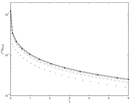
FIG. 1.: We show $t^{1/2}P(x,t)$ versus the scaling variable $\xi=x^{2}/t$ for the CTRW process. The curves in the figure are for the times $t=1,5,25,125$ (dots, dot dash, dashed, stared curve) respectively. We see that the CTRW solution converges in the limit of large times to the fractional diffusion approximation (solid line). The fractional solution diverges on the origin, hence it is cutoff in the figure. To find the exact solution we used Cauchy $\mu=1$ and Smirnov $\alpha=1/2$ stable laws. The results shown in Figs. $1-4$ were obtained using Mathematica.

A Diverging Solution of the Fractional Equation

We now investigate in detail the behavior of the CTRW and the corresponding fractional diffusion equation at the origin $x=0$. In Appendix A, the solution of the fractional diffusion equation is used to show that

$$P_{fr}(x,t)|_{x=0}=\left\{\begin{array}[]{c c}2^{1\over\mu}t^{-\alpha/\mu}{\Gamma\left(1-1/\mu\right)\over\Gamma\left(1-\alpha/\mu\right)}l_{\mu,0}(x)|_{x=0}&\mu>1\\ &\\ \infty&\mu\leq 1,\end{array}\right.$$ (14)

where $l_{\mu,0}(x)|_{x=0}=\Gamma(1/\mu)/(\mu\pi)$. The subscript fr stands for fractional diffusion approximation. We assumed $\alpha<1$ since the case $\alpha=1$ yields stable propagator $P_{fr}(x,t)$ which does not diverge on the origin (see Appendix A).

In Appendix B the exact CTRW solution, Eq. (7), is used to find the behavior of the CTRW on the origin (i.e. for the non singular terms). For $\alpha<1$ we find

$$P(x,t)|_{x=0}\sim\left\{\begin{array}[]{c c}2^{1/\mu}{\zeta\left({1\over\mu}\right)\over\Gamma(1-\alpha)}{1\over t^{\alpha}}l_{\mu,0}(x)|_{x=0}&\mu<1\\ &\\ {2\alpha\over\pi\Gamma(1-\alpha)}{\ln(t)-\hat{\psi}(\alpha)\over t^{\alpha}}&\mu=1\\ &\\ 2^{1/\mu}{\Gamma\left(1-1/\mu\right)\over\Gamma\left(1-\alpha/\mu\right)}{1\over t^{\alpha/\mu}}l_{\mu,0}(x)|_{x=0}&\mu>1,\end{array}\right.$$ (15)

where $\zeta(z)$ is the Riemann zeta function and $\hat{\psi}(\alpha)$ is the psi function [of course not related to $\psi(t)$]. In Fig. (2) we show $P(x,t)|_{x=0}$ versus $t$ for $\mu=1$, exhibiting how the exact CTRW solution converges to its asymptotic limit at the origin. Comparing Eq. (15) with Eq. (14) we see that the infinity found for $\mu\leq 1$ within the fractional framework is not related to the underlying CTRW. As mentioned, this shortcoming within the fractional approximation is due to the fact that number of steps in the random walk is an integer which cannot generally be approximated with a continuum approach [i.e., replacement of summation with integration in Eq. (7) is not justified for $0<\mu\leq 1$ in the vicinity of the origin]. In Fig. 2 we also show the approximation based on the Euler-Mclaurin formula Eq. (11). In contrast to the fractional diffusion approximation, Eq. (11) yields good agreement with the exact results. Note that divergence of the solution of the $d>1$ dimensional fractional diffusion equation with $\mu=2,\alpha<1$ (i.e. sub diffusive case) at the origin was discussed in [10, 34]. For these cases the exact CTRW solution is a valuable tool.

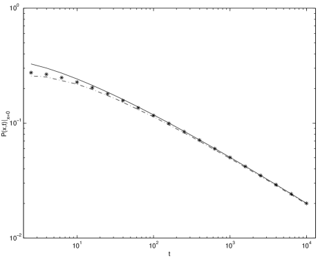
FIG. 2.: The behavior of exact CTRW on the origin, $P(x,t)|_{x=0}$ versus $t$ on log log plot for the case $\alpha=1/2$ and $\mu=1$. Not shown is the delta function contribution. The stars are the exact solution (7) while the solid curve is the asymptotic behavior Eq. (15). The fractional diffusion equation yields for this case $P(x,t)|_{x=0}=\infty$ and hence is invalid. The approximation based on the Euler–Mclaurin formula, Eq. (11), is the dot dashed curve. It yields good agreement with the exact results.

B Slow Convergence Toward Fractional Approximation

Let us consider as an example the case $\alpha=1/3$ and $\mu=2$. In Fig. 3 we show the exact CTRW solution in scaling form. As expected, for long times the CTRW solution seems to converge toward the solution of the fractional diffusion equation, though clear deviations of the CTRW solution from the fractional approximation are seen in the vicinity of the origin. In Fig. 4, a closer look at the behavior at the origin is presented. The figure shows that the CTRW convergence toward the fractional diffusion approximation is extremely slow, for $t=10^{13}$ deviations from asymptotic behavior are still observed (note that since $\psi(u)=\exp(-u^{1/3})$ the natural time unit is $1$, though the mean time between jumps diverges). Our improved approximation, Eq. (11), yields a good description of the underlying CTRW for intermediate and long times. We note that as $\alpha\to 0$ convergence of the CTRW solution toward the fractional approximation is expected to become much slower. And of course when $\alpha\to 1$, convergence becomes faster, though then deviations from Gaussian behavior $(i.e.,\mu=2,\alpha=1$) become small.

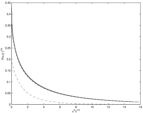
FIG. 3.: The long time convergence of the exact CTRW solution toward the fractional diffusion approximation for $\alpha=1/3$ and $\mu=2$. We present $t^{1/6}P(x,t)$ versus the scaling variable $x^{2}/t^{1/3}$. The CTRW curves in the figure are for the times $t=125,625,3125$ (dot dash, dashed, dot) respectively, the solution of the fractional diffusion equation is the solid line. To obtain the exact CTRW solution we use the waiting time density $l_{1/3,1}(t)=1/(3\pi)t^{-3/2}K_{1/3}\left({2\over\sqrt{27t}}\right)$, where $K_{1/3}$ is the modified Bessel function of the second kind. The jump length probability density is Gaussian $f(\delta x)=(4\pi)^{-1/2}\exp(-\delta x^{2}/4)$. For $\alpha=1/3$ and $\mu=2$ the solution of the fractional diffusion equation is $P(x,t)=3|x|^{-1}\xi l_{1/6,1}(\xi)$ with $\xi=t/|x|^{6}$.

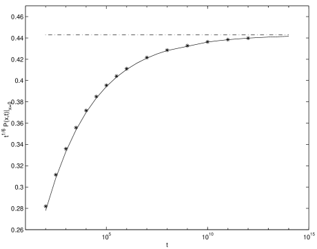
FIG. 4.: The very slow convergence of the non singular CTRW solution toward the fractional approximation on the origin. We use the same parameters as in Fig. 3. The exact CTRW solution are the stars, the dot dash line is the fractional approximation, and the solid curve is the approximation based on the Euler–Mclaurin formula, Eq. (11).

III The General Approach

While the exact solution presented in previous section gives insight into the validity of the fractional diffusion equation it is based on a particular choice of $\psi(t)$ and $f(\delta x)$. Here we shall consider a more general approach.

Let $P(x,t)$ describe a normalized Green function of an unspecified one dimensional random walk; later we treat specific examples in some detail. We shall use the convention that the arguments in the parenthesis define the space we are working in, thus $P(k,u)$ is the Fourier–Laplace transform of the Green function $P(x,t)$. It is assumed that $P(k,u)$ is known exactly as is the case for different types of CTRWs and for generalized master equations of the type investigated in [33].

Consider the expansion

$$P(k,u)=\sum_{n=0}^{\infty}M_{n}(u){(ik)^{n}\over n!},$$ (16)

where it is assumed that all the moments of the random walk

$$M_{n}(u)=\left({d\over idk}\right)^{n}P(k,u)|_{k=0}$$ (17)

are finite. The case when the moments diverge will be discussed later. According to Tauberian theorems [18, 29], the small $u$ behavior of the moments in the Laplace domain yield the long time behavior of the moments in the time domain. Namely, if $M_{n}(u)\sim c_{n}u^{-\xi_{n}-1}$ when $u\to 0$ then $M_{n}(t)\sim c_{n}t^{\xi_{n}}/\Gamma(1+\xi_{n})$ for $t\to\infty$, where $\xi_{n}>0$ and $c_{n}$ are constants. Our goal is to find the asymptotic moment generating function $P_{AMG}(k,u)$ which contains all the information on the $u\to 0$ behavior of the moments. We define this function according to

$$P_{AMG}(k,u)\equiv\sum_{n=0}^{\infty}c_{n}u^{-\xi_{n}-1}{\left(ik\right)^{n}\over n!}.$$ (18)

If this series can be summed (see examples to follow) the function $P_{AMG}(k,u)$ yields in a compact way all the asymptotic information on the moments of the underlying transport process. If the inverse Laplace–Fourier transform of $P_{AMG}(k,u)$ is a normalized non-negative probability density, then it is safe to say that $P_{AMG}(k,u)$ is the Fourier-Laplace transform of the asymptotic Green function i.e., $P(x,t)$ in the long time limit. This is the case for most Gaussian transport systems. Below we discuss Lévy walks where $P_{AMG}(k,u)$ does not yield the Green function $P(x,t)$ in the long time limit, even though it does contains all the information on the long time behavior of the moments.

IV Sub–Diffusion

We now consider as an example the well known decoupled continuous time random walk in the sub diffusive regime. Similar to previous work (e.g. [18]) we assume

$$\psi(u)=1-Au^{\alpha}+c_{1}u^{2\alpha}\cdots\ \ \ 0<\alpha<1,$$ (19)

for $u\to 0$, so that $\psi(t)\propto t^{-(1+\alpha)}$ for $t\to\infty$; hence $\psi(t)$ is moment-less. In what follows we use $A=1$ restoring $A$ only when it is important. We also assume

$$f(k)=1-{k^{2}\over 2}+{m_{4}k^{4}\over 4!}-{m_{6}k^{6}\over 6!}\cdots,$$ (20)

where $m_{i}$ are the finite moments of the PDF $f(\delta x)$. We assumed the $f(\delta x)$ is symmetric hence $m_{2i+1}=0$, the second moment being $m_{2}=1$. As discussed below some of these assumptions can be relaxed.

The Green function $P(x,t)$ of finding the random walker at $x$ at time $t$ is given in Fourier–Laplace space according to [18]

$$P(k,u)={1-\psi(u)\over u}{1\over 1-\psi(u)f(k)}.$$ (21)

The long time behavior of this equation is usually investigated based on the long wave length approximation (e.g., [13]), namely by inserting

$$\psi(u)f(k)=1-u^{\alpha}-{k^{2}\over 2}$$ (22)

and $\psi(u)=1-u^{\alpha}$ in Eq. (21). This approach implicitly assumes that simple scaling Eq. (3) with $\mu=2$ holds. Let us now see why this is the case.

We expand $P(k,u)$ in $k$

$$P(k,u)={1\over u}\left\{1-\Omega(u){k^{2}\over 2}+\left[6\Omega^{2}(u)+m_{4}\Omega(u)\right]{k^{4}\over 4!}-\right.$$

$$\left.\left[90\Omega^{3}(u)+30m_{4}\Omega^{2}(u)+m_{6}\Omega(u)\right]{k^{6}\over 6!}\cdots\right\}$$ (23)

where $\Omega(u)=\psi(u)/[1-\psi(u)]$. The $i$ th term in the expansion gives the moment $M_{i}(u)$ of the random walker in-terms of the “microscopic” moments $m_{i}$ and $\Omega(u)$. For example $M_{0}=1/u$ which means that the normalization is conserved, $M_{2}(u)=\Omega(u)/u$ etc. In the long wave length approximation (or in the fractional diffusion equation approach) one sets $m_{i}=0$ for $i\geq 4$. To see why and when this works well we must consider the high order moments $M_{i}$ and $i\geq 4$. For example

$$M_{4}(u)={\left[6\Omega^{2}(u)+m_{4}\Omega(u)\right]\over u}.$$ (24)

We now consider the $u\to 0$ limit of this expression since this limit will yield the asymptotic expression for $M_{4}(t)$ when $t\to\infty$. Using $\Omega(u)\sim 1/u^{\alpha}$ it is easy to see that

$$M_{4}(u)\sim{6\over u^{1+2\alpha}},$$ (25)

and we see that $M_{4}(u)$ is independent of $m_{4}$ in the limit $u\to 0$. Similar behavior is found for all the higher order moments

$$M_{2j}(u)\sim{1\over u}{\left(2j\right)!\over\left(2u^{\alpha}\right)^{j}},$$ (26)

which is independent of $c_{1}$ and $m_{2j}$ for $j>1$. This behavior is similar in some sense to normal (i.e., $\alpha=1$) random walk where all the moments $M_{n}(u)$ converge in a limit to simple Gaussian behavior which is independent of the details of the underlying random walks. However now we are not considering Gaussian diffusion. It is also easy to show that behavior in Eq. (26) is compatible with the scaling assumption Eq. (3). Using Eq. (18) one finds

$$P_{AMG}(k,u)=\sum_{j=0}^{\infty}{k^{2j}(-1)^{j}\over u(2u^{\alpha})^{j}},$$ (27)

summing this geometric series we have

$$P_{AMG}(k,u)={u^{\alpha-1}\over u^{\alpha}+k^{2}/2}.$$ (28)

Or we may inverse Laplace transform Eq. (27) term by term and find

$$P_{AMG}(k,t)=\sum_{j=0}^{\infty}\left({-k^{2}\over 2}\right)^{j}{t^{\alpha j}\over\Gamma\left(1+\alpha j\right)}=E_{\alpha}\left(-{k^{2}t^{\alpha}\over 2}\right),$$ (29)

where $E_{\alpha}(x)$ is the Mittag-Leffler function. Since Eq. (28) is the Fourier Laplace transform of a non negative probability density (see e.g. Appendix A), it yields $P(x,t)$ in the long time limit.

Eq. (28) is the Fourier–Laplace transform of the fractional diffusion equation (1) when $\mu=2$ and $0<\alpha<1$, and well known within the CTRW community [21]. The inverse Fourier–Laplace transform of Eq. (28) was investigated in [5, 10, 35] in dimensions $d=1,2,3$. Here we showed that: $(i)$ this equation does indeed describe the long time behavior of the moments of the random walk to all orders and $(ii)$ that these moments depend only on three parameters of the model $\alpha,m_{2}=1$ and $A=1$ (i.e., universality) . Our approach clarifies the usual long wave length approximation which is based on the exact calculation of only the first two moments. In the following section we will discuss coupled memories where the asymptotic behavior is not as straightforward as for the decoupled case.

In our derivation we assumed that start of observation and start of the process coincide. If the first step is described by $\psi_{1}(t)\neq\psi(t)$, one can show that our results are still valid for $\psi_{1}(t)$ decaying faster then $\psi_{1}(t)\propto t^{-(1+\beta)}$, with $\beta>0$. When $\beta<<\alpha$ the convergence becomes slow. If the random walk is biased, $m_{1}\neq 0$, one can easily show that biased fractional diffusion equation (e.g. [10]) holds in the long time limit.

V Enhanced–Diffusion

We now consider an example exhibiting enhanced, Lévy walk type of diffusion. We start by introducing the coupled CTRW jump model, investigated by Zumofen, Klafter and Shlesinger [36, 37] in the context of chaotic maps. Such a random walk is also related to transport in random media [38, 39], tracer diffusion in turbulent flow [40] and to the blinking of Quantum dots [41]. Closely related models are the velocity models investigated in [36, 42, 43, 44].

In CTRW the random walk is entirely specified by $\tilde{\psi}(\delta x,t)$, the probability density to move a distance $\delta x$ in time $t$ in a single jump event. For the jump model a coupled space-time memory is assumed

$$\tilde{\psi}\left(\delta x,t\right)={1\over 2}\delta\left(|\delta x|-t\right)\psi(t).$$ (30)

Such a model describes a particle trapped on the origin for time $t_{1}$ then it jumps to a new location whose distance from the origin is $|\delta x|=t_{1}$ (i.e, $x_{1}=\pm t_{1}$ with equal probability), then the process is renewed. From Eq. (30) we see that the random times $\{t_{i}\}$ are distributed according to $\psi(t)$ and the length of each jump $i$ is $|\delta x_{i}|=t_{i}$. Hence a large jump will “cost” a long time. This is different from the Lévy flight model where jumps on all scales are performed at constant time intervals. Thus in some applications Lévy walks are considered more physical than Lévy flights; however, as discussed below these two models are in fact deeply related. The space time coupling in Eq. (30) guarantees that for the Lévy walk model, $P(x,t)=0$ for $|x|>t$, this in turn implies that all moments of the random walk are finite. For Lévy flights even moments diverge.

The Laplace–Fourier transform of the Lévy walk Green function is [36]

$$P(k,u)={1-\psi(u)\over u\left[1-\tilde{\psi}\left(u,k\right)\right]}$$ (31)

where

$$\tilde{\psi}(k,u)=\int_{0}^{\infty}dte^{-ut}\cos\left(kt\right)\psi(t).$$ (32)

The moments of the random walk are now calculated using Eq. (31) and Mathematica, one finds $M_{0}(u)=1/u$

$$M_{2}(u)={1\over u}{\psi^{(2)}(u)\over 1-\psi(u)}$$

$$M_{4}(u)={1\over u}{\left[1-\psi(u)\right]\psi^{(4)}(u)+6\left[\psi^{(2)}\left(u\right)\right]^{2}\over\left[1-\psi(u)\right]^{2}}$$ (33)

where $\psi^{(2j)}(u)$ is the $2j$ th derivative of $\psi(u)$ with respect to $u$. Odd moments vanish due to the assumed symmetry of the random walk. Higher order moments are calculated in a similar way, for the sake of space they are not included here.

  

A Sub–Ballistic Enhanced Diffusion

Let as now consider $\psi(u)\sim 1-u\tau+Bu^{\beta}\cdots$ and $1<\beta<2$. Unlike the previous example, now the mean waiting time $\tau$ is finite and the second moment of the waiting time distribution diverges. The model exhibits enhanced diffusion $\langle x^{2}\rangle\propto t^{\alpha}$ and $\alpha=3-\beta$.

As we shall see in detail, the model exhibits a strong type of anomalous diffusion. By definition [27] strong anomalous diffusion behavior exhibits $M_{2j}(t)\propto t^{f(j)}$ where $f(j)$ is a non–linear function of $j$ (see related work [38, 47, 48]). Castiglione et al [27] point out that strong anomalous diffusion implies the failure of the standard scaling assumption Eq. (3), since this equation predicts $M_{2j}(t)\propto t^{\alpha j}$ a behavior called weak anomalous diffusion.

Castiglione et al argue quite generally that a dynamical system exhibiting strong anomalous diffusion cannot be described by fractional diffusion equation. We show below, based on work of Zumofen et al [24] and others, that the Green function $P(x,t)$ is well described by the fractional diffusion approximation.

First we consider a long wave length approximation, and show the relation between this approximation and the fractional diffusion framework. We rewrite Eq. (31) in the form

$$uP(k,u)-u\tilde{\psi}(k,u)P(k,u)=1-\psi(u).$$ (34)

Due to Tauberian theorems, the behavior of $P(x,t)$ for $t\to\infty$ is controlled by the behavior of $P(k,u)$ at $u\to 0$, hence in the small $u$ limit (and fixed $k$) one finds

$$P(k,u)\left\{1-\left[\tilde{\psi}(k,u)|_{u=0}-u\int_{0}^{\infty}t\cos\left(kt\right)\psi(t)dt+\cdots\right]\right\}=$$

$$\tau-Bu^{\beta-1}+\cdots.$$ (35)

We now consider the $k\to 0$ limit using $\tilde{\psi}(k,u)|_{u=0}=1+B|k|^{\beta}\cos\left(\pi\beta/2\right)+\cdots$ leading to

$$P(k,u)\approx{1\over u+B|k|^{\beta}|\cos\left(\pi\beta/2\right)|/\tau}.$$ (36)

Eq. (36) is rewritten in terms of a fractional diffusion equation using convenient units

$${\partial P_{fr}(x,t)\over\partial t}-{1\over 2}{\partial^{\beta}\over\partial|x|^{\beta}}P_{fr}(x,t)=\delta(x)\delta(t).$$ (37)

Eq. (37) describes Lévy flights, whose solution is a symmetric Lévy stable PDF given in Appendix A, Eq. (51). The derivation of Eq. (37) based on the long wave length approximation is not rigorous; however Zumofen et al [24] used a numerical inverse Fourier–Laplace technique to show that the propagator is well described by a Lévy stable PDF. This result was verified by several authors, Araujo et al [43] used a numerically exact enumeration technique [49] and Mantegna [45] and Weron and Weron [46] used a Monte Carlo approach. As briefly mentioned in the introduction Kotulsky [26] used a rigorous limit theorem approach to reach the same conclusion. Thus in contradiction to the claim made in [27], the fractional equation yields a meaningful approximation to the underlying strong anomalous diffusion process under investigation.

We are still left with a puzzle: the fractional equation predicts a non analytical behavior of $P(k,u)$, namely the divergence of the even moments of the random walk, while we know that these moments, for any finite time are finite. Let us therefore investigate the moments in greater detail, using Eq. (33) $M_{0}(u)=1/u$ and for $j\geq 1$,

$$M_{2j}(u)\sim{B\over\tau}\Theta_{2j}(\beta)u^{\beta-2-2j},$$ (38)

where $\Theta_{2j}(\beta)\equiv\Pi_{l=0}^{2j-1}|l-\beta|$. Inverting to the time domain we find the mentioned strong type of anomalous diffusion $M_{2j}(t)\propto t^{2j+1-\beta}$ for $j=1,2\cdots$ while $M_{0}=1$. We now investigate the behavior of the asymptotic moment generating function, based on the method in Sec. III. According to Eq. (18)

$$P_{AMG}(k,u)={1\over u}+{B\over\tau}u^{\beta-2}\sum_{j=1}^{\infty}\left(-{k^{2}\over u^{2}}\right)^{j}{\Theta_{2j}\left(\beta\right)\over\left(2j\right)!},$$ (39)

using the identity (obtained using Mathematica)

$$g(x)\equiv$$

$$\sum_{j=1}^{\infty}\left(-x\right)^{j}{\Theta_{2j}\left(\beta\right)\over\left(2j\right)!}=-1+(1+x)^{\beta/2}\cos\left[\beta\arctan\left(\sqrt{x}\right)\right],$$ (40)

we find

$$P_{AMG}(k,u)={1\over u}+{B\over\tau}u^{\beta-2}g({k^{2}\over u^{2}}).$$ (41)

We note that unlike the sub diffusive case, $P_{AMG}(k,u)$ Eq. (41) is not the Fourier Laplace transform of the asymptotic $P(x,t)$ since $\lim_{k\to\infty}P_{AMG}(k,u)=\infty$, when $u$ is fixed.

To conclude, according to long-wave length approximation and previous work, the jump model propagator $P(x,t)$ is described by the fractional diffusion equation with ($\alpha=1,\mu=\beta$). This approximation does not describe the behavior of the moments of the underlying random walk including the second. These are described by the moment generating function Eq. (41); thus, two functions yield the details on the long time behavior of the underlying random walk. And strong anomalous diffusion does not necessarily imply the breakdown of the fractional approximation, though one should take care in the interpretation of the results obtained by it.

A similar situation occurs in the field of inhomogeneous line broadening [50], where the line is well approximated by Lévy stable densities [51] (due to long range interactions between defects and chromophores). However (due to cutoffs) even moments of the line exist [50]. As discussed by Stoneham [50] these moments are sensitive to behavior of the line in its wings, and hence in the usual experimental situation (in the field of line broadening) are not considered relevant.

B Ballistic Diffusion

We now briefly consider the jump model with $\psi(u)=1-u^{\beta}\cdots$, with $0<\beta<1$. For this case the model exhibits ballistic diffusion $\langle x^{2}(t)\rangle\propto t^{2}$ [24]. Without going into details, we find the asymptotic moment generating function

$$P_{AMG}(k,u)={2u^{\beta-1}\over\left(u+ik\right)^{\beta}+\left(u-ik\right)^{\beta}}.$$ (42)

Zumofen et al [24] used an expansion in the small parameter $u\pm ik$ and numerical simulation for $\beta=1/2$, showing that Eq. (42) describes well long time behavior of $P(x,t)$ (at least for $\beta=1/2$). Here we showed that the approximation in [24], yields the behavior of the moments to infinite order. Eq. (42) is not related to a known fractional diffusion equation. Note that the fractional diffusion equation in the ballistic limit $\mu=2,\alpha=2$ yields the wave equation.

VI Lévy Flights with Long Rests

We now consider decoupled CTRW, where $\tilde{\psi}(\delta x,t)=\psi(t)f(\delta x)$, assuming the moments of $f(\delta x)$ diverge. Clearly, now the general approach presented in Sec. III breaks down and a generalization is now considered. We assume

$$f(k)=1-{|k|^{\mu}\over 2}+{a_{2\mu}|k|^{2\mu}\over 4!}-{a_{3\mu}|k|^{3\mu}\over 4!}+\cdots$$ (43)

and $0<\mu<2$. The coefficients $a_{j\mu}$ are called the amplitudes of the PDF $f(\delta x)$. An example being the symmetric stable densities $f(k)=l_{\mu,0}(k/\sqrt{2})$ where $l_{\mu,0}(k)\equiv\exp(-|k|^{\mu})$. We assume as before that

$$\psi(u)=1-u^{\alpha}+c_{1}u^{2\alpha}\cdots\ \ \ 0<\alpha<1,$$ (44)

for $u\to 0$, then using Eq. (21)

$$P(k,u)={1\over u}\left\{1-\Omega(u){|k|^{\mu}\over 2}+\left[6\Omega^{2}(u)+a_{2\mu}\Omega(u)\right]{|k|^{2\mu}\over 4!}-\right.$$

$$\left.\left[90\Omega^{3}(u)+30a_{2\mu}\Omega^{2}(u)+a_{3\mu}\Omega(u)\right]{|k|^{3\mu}\over 6!}\cdots\right\}.$$ (45)

This equation has a structure similar to Eq. (23), we see that the amplitudes $a_{j\mu}$ are natural generalizations of the moments $m_{2j}$. We define the amplitudes $A_{j\mu}(t)$ according to

$$P(k,u)=\sum_{j=0}^{\infty}(-1)^{j}{A_{j\mu}(u)|k|^{\mu j}\over(2j)!},$$ (46)

it follows from the discussion in Sec. IV that in the limit $u\to 0$, $A_{j\mu}(u)\sim(2j)!/(2^{j}u^{j\alpha+1})$. We define the amplitude generating function, in the spirit of Eq. (18), according to

$$P_{AG}(k,u)=\sum_{j=0}^{\infty}(-1)^{j}{|k|^{\mu j}\over 2^{j}u^{j\alpha+1}},$$ (47)

and it is easy to show that

$$P_{AG}(k,u)={u^{\alpha-1}\over u^{\alpha}+|k|^{\mu}/2}.$$ (48)

The right hand side of Eq. (48) is the Fourier-Laplace transform of the fractional diffusion equation (1). Hence the fractional equation describes the amplitudes of the random walk in the limit $t\to\infty$. However this does not necessarily imply that for all $x$ the corresponding $P(x,t)$ describes the CTRW in the limit $t\to\infty$. As shown already in subsection II A, for $\mu\leq 1$ and on the origin where $P(x,t)$ attains its maximum, the CTRW solution and the fractional diffusion equation solution are different. This limitation of the fractional equation is related to the fact that it is based on a small $k$ expansion which implies large $x$ behavior. Note that Eq. (48) was recently suggested by Kutner [52] to describe a Weierstrass flight.

VII Discussion

The fractional diffusion equation yields the asymptotic behavior of coupled and decoupled CTRWs. However the fractional approach has its limitations if compared with ordinary diffusion approximation. Careful analysis of the underlying random walk is needed for a better understanding of the domain of validity of the fractional equation. In particular the fractional approximation (for decoupled CTRWs) breaks down at the origin $x=0$ (for $\{0<\alpha<1\}\cap\{0<\mu\leq 1\}$). More generally the convergence of the CTRW solution, at $x=0$, toward the fractional approximation may become extremely slow. This behavior is different from ordinary random walks where (usually) (i) deviation from Gaussian behavior is found in the tails $|x|\to\infty$ (i.e., for long though finite times) and (ii) convergence toward the fractional approximation is typically fast. Also note that the fractional equation has a CTRW foundation only when $\{0<\alpha\leq 1\}\cap\{0<\mu\leq 2\}$ while the regime $\{1<\alpha\leq\mu\leq 2\}$ is not related to the CTRWs under investigation (see however work in [8] for $\{1<\alpha\leq 2=\mu\}$).

If they exist, moments of the decoupled CTRW converge in a long time limit to the behavior predicted by the fractional equation. For coupled memories describing Lévy walks the situation is more complicated. The fractional approximation describes the asymptotic long time behavior of the Green function $P(x,t)$, though it does not describe correctly the moments of the underlying random walk, not even the second moment. In this case we may characterize the random walk using both $P(x,t)$ and the asymptotic moment generating function. These two function yield different types of information, it is still to be seen if the asymptotic moment generating function has any universal features.

We note that a similar situation exists also for some simple random walks which are approximated with the ordinary diffusion equation. To see this consider as an example the sum of $N\to\infty$ independent, identically distributed random variables $\{x_{i}\}$, $i=1,2\cdots N$. As well known the sum $\sum_{i=1}^{N}x_{i}$ converges in a limit to a Gaussian behavior, provided the variance of $x_{i}$ exists. Assume the variance exists but higher order moments of $x_{i}$ diverge. Then clearly the central limit theorem, or identically the ordinary diffusion approximation, fails to predict correctly the behavior of the high order moments of the random walk (i.e., the Gaussian central limit theorem does not hold at the tails of the Green function). The situation for the fractional diffusion equation is similar to this case, in that it fails to predict correctly the behavior of the moments of the Lévy walk (i.e., the Lévy central limit theorem does not hold at the tails of the Green function of the Lévy walk, where $P(x,t)=0$ for $|x|>t$).

Note that our conclusions are valid only for free boundary conditions, for other boundary conditions we know little on domain of validity of the fractional diffusion equation especially when $\mu<2$ (see however work in [10, 53, 54]).

Acknowledgment: This research was supported in part by a grant from the NSF. I thank A. I. Saichev and G. Zumofen for helpful correspondence and R. Silbey for comments on the manuscript.

VIII Appendix A

We investigate the solution of fractional diffusion equation, with $\alpha\leq 1$ and $0<\mu\leq 2$. Following [6] we rewrite the solution in Fourier-Laplace space

$$P_{fr}(k,u)=u^{\alpha-1}\int_{0}^{\infty}dse^{-s\left(u^{\alpha}+|k|^{\mu}/2\right)}.$$ (49)

Since the symmetric Lévy stable probability density $l_{\mu,0}(x)$ and $\exp(-|k|^{\mu})$ are Fourier pairs

$$P_{fr}(x,u)=2^{1/\mu}u^{\alpha-1}\int_{0}^{\infty}dse^{-su^{\alpha}}l_{\mu,0}\left({2^{1/\mu}x\over s^{1/\mu}}\right)s^{-1/\mu}.$$ (50)

For $\alpha=1$ we use the Laplace pair $\exp(-su)$ and $\delta(t-s)$ and find as expected

$$P_{fr}(x,t)=\left({2^{1/\mu}\over t}\right)^{1\over\mu}l_{\mu,0}\left({2^{1/\mu}x\over t^{1/\mu}}\right),$$ (51)

and when $\mu=2$ the solution is Gaussian.

We now consider $\alpha<1$ and investigate the behavior on the origin. Using Eq. (50)

$$P_{fr}(x,u)|_{x=0}=2^{1/\mu}u^{\alpha-1}\int_{0}^{\infty}dss^{-1/\mu}e^{-su^{\alpha}}l_{\mu,0}\left(x\right)|_{x=0}$$ (52)

where $l_{\mu,0}(x)|_{x=0}=\Gamma(1/\mu)/(\mu\pi)$, we find

$$P_{fr}(x,u)|_{x=0}=\left\{\begin{array}[]{c c}2^{1/\mu}u^{\alpha/\mu-1}\Gamma\left(1-1/\mu\right)l_{\mu,0}\left(x\right)|_{x=0}&\mu>1\\ &\\ \infty&\mu\leq 1\end{array}\right.$$ (53)

which when inverted yields Eq. (14). For $\mu<1$, $P_{fr}(x,u)|_{x=0}$ is infinite due to the zero lower bound in the integral Eq. (52).

An integral solution of the fractional diffusion equation is found using the Laplace pair $u^{\alpha-1}\exp(-su^{\alpha})$ and $(1/\alpha)(t/s^{1+a/\alpha})l_{\alpha,0}(t/s^{1/\alpha})$ where $l_{\alpha,1}(t)$ is the one sided stable density whose Laplace transform is $\exp(-u^{\alpha})$. Hence

$$P_{fr}(x,t)=$$

$${2^{1/\mu}t\over\alpha}\int_{0}^{\infty}dss^{-(1+1/\alpha+1/\mu)}l_{\alpha,1}\left({t\over s^{1/\alpha}}\right)l_{\mu,0}\left({2^{1/\mu}x\over s^{1/\mu}}\right),$$ (54)

this equation being valid for $0<\alpha\leq 1$ and $0<\mu\leq 2$.

IX Appendix B

We investigate the CTRW solution

$$P(x,u)={1-e^{-u^{\alpha}}\over u}\delta(x)+$$

$$\left({1-e^{-u^{\alpha}}\over u}\right)\sum_{s=1}^{\infty}e^{su^{\alpha}}\left({2\over s}\right)^{1/\mu}l_{\mu,0}\left({2^{1/\mu}x\over s^{1/\mu}}\right).$$ (55)

The first term can be easily handled yielding $L_{\alpha,1}(t)\delta(x)$ decaying for long times like $\delta(x)t^{-\alpha}$. This singular term is neglected in the fractional diffusion approximation. Omitting this term we find for $x=0$,

$$P(x,u)|_{x=0}=$$

$$\left({1-e^{-u^{\alpha}}\over u}\right)\sum_{s=1}^{\infty}e^{-su^{\alpha}}\left({2\over s}\right)^{1/\mu}l_{\mu,0}\left(x\right)|_{x=0}=$$

$$2^{1/\mu}\left({1-e^{-u^{\alpha}}\over u}\right)\mbox{PolyLog}\left[{1\over\mu},e^{-u^{\alpha}}\right]l_{\mu,0}\left(x\right)|_{x=0}$$ (56)

where $\mbox{PolyLog}\left[n,z\right]$ is the $n$ th polylogarithm function of $z$. For $\mu<1$ and $u\to 0$ we find

$$P(x,u)|_{x=0}\sim 2^{1/\mu}u^{\alpha-1}\zeta\left({1\over\mu}\right)l_{\mu,0}(x)|_{x=0},$$ (57)

where $\zeta(z)$ is Riemann’s zeta function. For $\mu=1$ we use $\sum\exp(-su^{\alpha})/s=-\ln[1-\exp(-su^{\alpha})]$ to find

$$P(x,u)|_{x=0}\sim-2u^{\alpha-1}\ln\left(u^{\alpha}\right)l_{1,0}(x)|_{x=0}.$$ (58)

For $1<\mu<2$ we use the Euler–Mclaurin summation formula

$$\sum_{s=1}^{\infty}e^{-su^{\alpha}}s^{-1/\mu}=e^{-u^{\alpha}}\left[1+\sum_{k=1}^{\infty}e^{-ku^{\alpha}}(k+1)^{-1/\mu}\right]=$$

$$e^{-u^{\alpha}}\left[1+\int_{0}^{\infty}dk{e^{-ku^{\alpha}}\over\left(1+k\right)^{1/\mu}}-{1\over 2}+{1\over 12}{d\over dk}{e^{-ku^{\alpha}}\over\left(1+k\right)^{1/\mu}}|_{0}^{\infty}+\cdots\right]$$ (59)

where $\cdots$ are the higher order terms in the Euler–Mclaurin formula. The integral in Eq. (59) in the limit $u\to 0$ yields

$$\int_{0}^{\infty}dk{e^{-ku^{\alpha}}\over\left(1+k\right)^{1/\mu}}\sim u^{\alpha/\mu-\alpha}\Gamma\left(1-{1\over\mu}\right),$$ (60)

provided that $\mu>1$. This term is much larger than the other terms in Eq. (59); hence, we find

$$P(x,u)|_{x=0}\sim 2^{1/\mu}u^{\alpha/\mu-1}\Gamma\left(1-{1\over\mu}\right)l_{\mu,0}(x)|_{x=0}.$$ (61)

Inverting Eqs. (57,58,61) we find Eq. (15).

REFERENCES

- [1] S. G. Samko, A. A. Kilbas and O. I. Marichev Fractional Integrals and Derivatives Theory and Applications Gordon and Breach Science Publishers, (USA) 1993.
- [2] R. Hilfer, ….
- [3] www.fracalmo.org
- [4] S. Bochner, Proc. Nat. Acad. Sciences USA 35 368-370 (1949).
- [5] W. R. Schneider and W. Wyss, J. Math. Phys. 30, 134 (1989).
- [6] A. I. Saichev and M. Zaslavsky, Chaos 7, 753 (1997).
- [7] R. Metzler, E. Barkai and J. Klafter, Phys. Rev. Lett. 82, 3563 (1999).
- [8] E. Barkai, R. Silbey , J. Phys. Chem. B 3866 (2000).
- [9] V. V. Yanovsky, A. V. Chechkin, D. Schertzer, and A. V. Tur Physica (Amsterdam) 282A, 13 (2000).
- [10] E. Barkai, Phys. Rev. E 63,6304(4):6118 (2001).
- [11] E. Lutz Phys. Rev. Lett. 86, 2208 (2001).
- [12] H. Weitzner, and G. M. Zaslavsky Chaos 11, 384 (2001).
- [13] R. Metzler and J. Klafter, Phys. Rep. 339 1 (2000).
- [14] R. Hilfer and L. Anton, Phys. Rev. E. 51, R848 (1995).
- [15] A. Compte, Phys. Rev. E 53, 4191 (1996).
- [16] R. Metzler, I. Sokolov and J. Klafter, Phys. Rev. E 58, 1621 (1998).
- [17] E. Barkai, R. Metzler and J. Klafter, Phys. Rev. E. 61 132 (2000).
- [18] G. H. Weiss, Aspects and Applications of the Random Walk North Holland (Amsterdam – New York – Oxford, 1994).
- [19] I. M. Sokolov, A. Blumen, and J. Klafter Cond-mat 0107632
- [20] F. Mainardi, Y. Luchko, and G. Pagnini Fractional Calculus and Applied Analysis 4, 153 (2001)
- [21] J. K. E. Tunaley, J. of Stat. Mech. 11, 397 (1974).
- [22] M. F. Shlesinger, J. Klafter and Y. M. Wong, J. Stat. Phys. 27 499 (1 982).
- [23] J. Klafter, A. Blumen and M. F. Shlesinger, Phys. Rev. A 35, 3081 (1987).
- [24] G. Zumofen, J. Klafter, and A. Blumen Chemical Physics 146 433 (1990)
- [25] M. Kotulski, J. Stat. Phys. 81, 777 (1995).
- [26] M. Kotulski, Chaos the Interplay Between Stochastic and Deterministic Behavior Ed. P. Garbaczewski, M. Wolf and A. Weron, Lecture Notes in Physics, Vol. 457 (Springer) 1995 p. 471.
- [27] P. Castiglione, A. Mazzino, P. Muratore-Ginanneschi and A. Vulpiani Physica D 134 75 (1999).
- [28] W. R. Schneider in Stochastic Processes in Classical and Quantum Systems Eds. S. Albeverio, G. Casatti and D. Merlini (Lecture Notes in Physics, Springer, Berlin, 1986).
- [29] W. Feller,An introduction to probability Theory and Its Applications Vol. 2 (John Wiley and Sons 1970).
- [30] E. W. Montroll and J. T. Bendler, J. Stat. Phys. 34, 129 (1984)
- [31] Closed form expressions for Lévy stable PDFs, were obtained by Schneider [28], in terms of Fox H functions (i.e., for and ). However, only for special cases one finds a simple (i.e., tabulated and accessible) closed form expression for Lévy stable probability densities. Series expansions, and asymptotic behaviors of stable laws are summarized in [28]. Note that [28] also points out relevant errors in the literature. A brief summary of properties of one sided stable laws can also be found in an Appendix in [10].
- [32] Handbook of Mathematical Functions Edited by M. Abramowitz and I. A. Stegun (Dover Publications Inc) New York (1970)
- [33] R. Metzler, E. Barkai and J. Klafter, Europhys. Lett. 46 (4) 431 (1999).
- [34] R. Hilfer Fractals 3, 211 (1995).
- [35] J. Klafter and G. Zumofen, J. Phys. Chem. 98, 7366 (1994).
- [36] G. Zumofen and J. Klafter Phys. Rev. E 47 851 (1993)
- [37] J. Klafter, G. Zumofen and M. F. Shlesinger Chaos the Interplay Between Stochastic and Deterministic Behavior Ed. P. Garbaczewski, M. Wolf and A. Weron, Lecture Notes in Physics, Vol. 457 (Springer) 1995 p. 183.
- [38] E. Barkai, V. Fleurov, and J. Klafter Phys. Rev. E 61 1164 (2000).
- [39] P. Levitz, Europhys. Lett. 39 593 (1997).
- [40] T. H. Solomon, E. R. Weeks, and H. L. Swinney, Phys. Rev. Lett. 71, 3975 (1993).
- [41] Y. Jung, E. Barkai, R. Silbey (submitted).
- [42] J. Masoliver, K. Lindenberg, and G. H. Weiss, Physica A 157 891 (1989).
- [43] M. Araujo, S. Havlin, G. H. Weiss and H. E. Stanley Phys. Rev. A 43 5207 (1991).
- [44] E. Barkai and V. Fleurov, Phys. Rev. E. 56, 6355, (1997).
- [45] R. M. Mantegna J. Stat. Phys. 70 721 (1993).
- [46] A. Weron and R. Weron Chaos the Interplay Between Stochastic and Deterministic Behavior Ed. P. Garbaczewski, M. Wolf and A. Weron, Lecture Notes in Physics, Vol. 457 (Springer) 1995 p. 379.
- [47] K. H. Andersen, P. Castiglione, A. Mazzino, and A. Vulpiani Eur. Phys. J. B. 18 447 (2000).
- [48] B .A. Carreras, V.E. Lynch, D.E. Newman, and G. M. Zaslavsky, Phys. Rev. E 69 4770 (1999).
- [49] Araujo et al [43] use a closely related velocity model.
- [50] A. M. Stoneham, Rev. Mod. Phys. 41 82 (1969).
- [51] E. Barkai, R. Silbey, and G. Zumofen, J. Chem. Phys. 113 5853 (2000).
- [52] R. Kutner, Physica A 264 84 (1999).
- [53] G. Rangarajan and M. Z. Ding, Phys. Rev. E 62 120 (200).
- [54] S. V. Buldyrev et al Cond-mat article number 0012513.