Theory of electron spectroscopies

Abstract

The basic theory of photoemission, inverse photoemission, Auger-electron and appearance-potential spectroscopy is developed within a unified framework starting from Fermi’s golden rule. The spin-resolved and temperature-dependent appearance-potential spectroscopy of band-ferromagnetic transition metals is studied in detail. It is shown that the consideration of electron correlations and orbitally resolved transition-matrix elements is essential for a quantitative agreement with experiments for Ni.

1 Basic electron spectroscopies

Electron spectroscopy Pen74 ; PH74 ; FFW78 ; Fug81 ; Ram91 ; Don94 is one of the fundamental experimental techniques to investigate the electronic structure of transition metals. For a deeper understanding of the electronic properties, a meaningful interpretation of the measured spectra is necessary which is based on a reliable theory of spectroscopies. This is particularly important for the study of band ferromagnetism which is caused by a strong Coulomb interaction among the valence electrons. Due to the presence of strong electron correlations, simple explanations of spectral features within an independent-particle model may fail. Here we try to clarify what physical quantity is really measured and what ingredients are needed for a theoretical approach to find a satisfactory agreement with the experimental data. We are concerned with the theory of four basic types of electron spectroscopy (see Fig. 1): photoemission (PES), inverse photoemission (IPE), Auger-electron (AES) and appearance-potential spectroscopy (APS).

The spin-, angle- and energy-resolved (ultraviolet) valence-band photoemission (PES) more or less directly measures the occupied part of the band structure. Present theories of PES are mostly based on the so-called one-step model of photoemission Pen74 ; Pen76 ; Bor85 ; Bra96 which treats the initial excitation step, the transport of the photoelectron to the surface and the scattering at the surface barrier as a single quantum-mechanically coherent process. The one-step model is essentially based on the independent-particle approximation. The valence electrons move independently in an effective potential as obtained from band-structure calculations within the local-density approximation (LDA) of density-functional theory (DFT) HK64 ; KS65 . There are recent attempts PLNB97 ; MPN+99 for a reformulation of the one-step model to include a non-local, complex and energy-dependent self-energy which accounts for electron correlations.

The one-step model also applies to inverse photoemission spectroscopy. IPE is complementary to PES and yields information on the unoccupied bands above the Fermi energy Bra96 . For example, IPE can be used to determine the dispersions of the Rydberg-like series of surface states in the $1/z$ image potential in front of the surface Don94 .

The theory of CVV Auger-electron spectroscopy (AES) is more complicated compared to PES/IPE since there are two valence electrons participating in the transition. Due to core state involved additionally, AES is highly element specific. This feature is frequently exploited for surface characterization. Contrary to $\bf k$ resolved (inverse) photoemission, the Auger transition is more or less localized in real space. High-resolution AES may thus yield valuable information on the local valence density of states (DOS). In the most simple theoretical approach suggested by Lander in 1953 Lan53 , the Auger spectrum is given by the self-convolution of the occupied part of the DOS. Modern theories of AES also include the effect of transition-matrix elements HWMR88 . Similar as the one-step model of PES and IPE, these approaches are based on the independent-electron approximation.

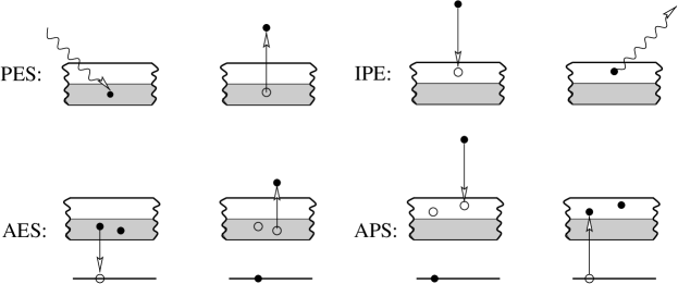
Figure 1: Schematic picture of the initial and the final states for different electron spectroscopies. PES: photoemission spectroscopy ($s=1$). IPE: inverse photoemission ($s=-1$). AES: Auger-electron spectroscopy ($s=2$). APS: appearance-potential spectroscopy ($s=-2$). The grey region is the occupied part of the valence band

Finally, the appearance-potential spectroscopy (APS) is complementary to AES. Within Lander’s independent-electron model Lan53 the AP line shape resulting from CVV transitions is given by the self-convolution of the unoccupied part of the DOS. Matrix elements are included in refined independent-particle theories EP97 . Its comparatively simple experimental setup and its surface sensitivity qualifies APS to study surface magnetism, for example. For a ferromagnetic material, the spin dependence of the AP signal obtained by using a polarized electron beam gives an estimate of the surface magnetization as has been demonstrated for the transition metals Fe and Ni Kir84 ; EVDN93 .

Common to all four spectroscopies are a number of fundamental concepts and approximation schemes used in the theoretical description. Therefore, it should be possible to develop the basic theory of PES, IPE, AES and APS within a unified framework. This is discussed in the following section 2. As a result of this basic theory of electron spectroscopies it found that in each case the intensity is essentially given in terms of a characteristic Green function.

The actual evaluation of the Green function is more specific and depends on the respective spectroscopy, on the material and the physical question to be investigated. In section 3 we will therefore pick up an example and give a more detailed discussion of APS for band ferro-magnets.

A notable quality of APS is its direct sensitivity to electron correlations: In the AP transition, two valence electrons are added to the system at a certain lattice site. These final-state electrons mutually experience the strong intra-atomic Coulomb interaction $U$. As a consequence the two-particle (AP) excitation spectrum is expected to show up a pronounced spectral-weight transfer or even a satellite with a characteristic energy of the order of $U$ Cin77 ; Saw77 . This is an important difference between the one- (PES, IPE) and the two-particle spectroscopies (AES, APS). To demonstrate this sensitivity to correlations in APS we consider the spin- and temperature-dependent AP spectra of ferromagnetic Nickel as a prototype of a strongly correlated and band-ferromagnetic material in section 4. The discussion of the calculations and the comparison with experimental results will show what presently can be achieved in the theory of electron spectroscopies. Some conclusions are given in section 5.

2 Theory

The basic theory starts from the Hamiltonian $H$ which shall describe the electronic structure of the system within a certain energy range around the Fermi energy. In addition, we consider a perturbation $V_{s}$ that mediates the respective transition. $V_{s}$ is assumed to be small and will be treated in lowest-order perturbation theory. The index $s$ distinguishes the different spectroscopies (see Fig. 1). $s=\pm 1,\pm 2$ stands for the difference between the number of valence electrons before and after the transition.

In the photoemission spectroscopy (PES, $s=+1$) a valence electron is excited into a high-energy scattering state by absorption of a photon. The photoelectron escapes into the vacuum and is captured by a detector depending on its spin, energy and angles relative to the crystal surface. Within the framework of second quantization, the perturbation can be written as:

$$V_{+1}=\sum_{\alpha\gamma}M_{\alpha\gamma}\,a^{\dagger}_{\alpha}c_{\gamma}+\mbox{h.c.}\qquad\mbox{(PES)}\>.$$ (1)

$c_{\gamma}$ annihilates a valence electron with quantum numbers $\gamma$, and $a_{\alpha}^{\dagger}$ creates an electron in a high-energy scattering state $\alpha$. The matrix element is calculated using the electric dipole approximation. This is well justified in the visible and ultraviolet spectral range. Neglecting the term quadratic in the field as usual and choosing the Coulomb gauge, one obtains:

$$M_{\alpha\gamma}=\langle\alpha|{\bf A}_{0}{\bf p}|\gamma\rangle\qquad(s=\pm 1)\>.$$ (2)

Here $\bf p$ is the momentum operator and ${\bf A}_{0}$ is the spatially constant vector potential inside the crystal. It can be determined from classical macroscopic dielectric theory. Note that we use atomic units with $e=m_{\rm e}=\hbar=1$.

In an inverse-photoemission experiment (IPE, $s=-1$) an electron beam characterized by quantum numbers $\alpha$ hits the crystal surface. An electron may be de-excited into an empty valence state $\gamma$ above the Fermi energy by emission of a photon. The photon yield is measured as a function of $\alpha$ (the polarization, the energy and the angles of the incident electron beam). We have:

$$V_{-1}=\sum_{\gamma\alpha}M_{\gamma\alpha}^{\ast}\,c^{\dagger}_{\gamma}a_{\alpha}+\mbox{h.c.}\qquad\mbox{(IPE)}\>.$$ (3)

Obviously, $V_{-1}=V_{1}$. Both, PES and IPE, are induced by the same electron-photon interaction.

In the case of the two-particle ($s=\pm 2$) spectroscopies AES and APS, the transitions are radiationless. Here the Coulomb interaction mediates between the initial and the final state. The initial state for AES ($s=+2$) is characterized by a hole in a core level (produced by a preceding core-electron excitation via x-ray absorption, for example). In the Auger transition the empty core state $\beta$ is filled by an electron from a valence state $\gamma$. The energy difference is transferred to another valence electron in the state $\gamma^{\prime}$ which is excited into a high-energy scattering state $\alpha$ and detected. Thus,

$$V_{+2}=\sum_{\alpha\beta\gamma^{\prime}\gamma}M_{\alpha\beta\gamma^{\prime}\gamma}\,a^{\dagger}_{\alpha}b^{\dagger}_{\beta}c_{\gamma}c_{\gamma^{\prime}}+\mbox{h.c.}\qquad\mbox{(AES)}\>.$$ (4)

The creator $b^{\dagger}_{\beta}$ refers to the core state.

Finally, an electron ($\alpha$) approaching the crystal surface can excite a core electron ($\beta$) into a state of the unoccupied bands. Above a threshold energy both, the de-excited primary electron and the excited core electron occupy valence states ($\gamma$, $\gamma^{\prime}$) above the Fermi energy after the transition. The appearance-potential spectroscopy (APS, $s=-2$) monitors the intensity of this transition as a function of polarization, energy and momentum of the incoming electron beam by detecting the emitted x-rays or Auger electrons of the subsequent core-hole decay. The perturbation is:

$$V_{-2}=\sum_{\alpha\beta\gamma^{\prime}\gamma}M_{\gamma^{\prime}\gamma\alpha\beta}^{\ast}\,c^{\dagger}_{\gamma^{\prime}}c^{\dagger}_{\gamma}b_{\beta}a_{\alpha}+\mbox{h.c.}\qquad\mbox{(APS)}\>.$$ (5)

Again, $V_{-2}=V_{2}$. Since AES and APS are induced by the Coulomb interaction, the matrix element reads:

$$M_{\alpha\beta\gamma^{\prime}\gamma}={}^{(1)}\!\langle\alpha|\,{}^{(2)}\!\langle\beta|\>\frac{1}{|{\bf r}_{1}-{\bf r}_{2}|}\>|\gamma^{\prime}\rangle^{(1)}\,|\gamma\rangle^{(2)}\qquad(s=\pm 2)\>.$$ (6)

To calculate the cross sections for the different spectroscopies, time-dependent perturbation theory with respect to the perturbation $V_{s}$ is applied. Using Fermi’s golden rule, the transition probability per unit time for a transition from the initial state $|E_{i}\rangle$ to the final state $|E_{f}\rangle$ is given by:

$$w_{s}=2\pi\,|\langle E_{f}|V_{s}|E_{i}\rangle|^{2}\,\delta(E_{f}-E_{i}-\omega_{s})\>.$$ (7)

$|E_{i}\rangle$ and $|E_{f}\rangle$ are eigenstates of the grand-canonical Hamiltonian $H-\mu N$ with eigenenergies $E_{i}$ and $E_{f}$. $\mu$ is the chemical potential and $N$ the particle-number operator. Furthermore, $\omega_{s}=\pm\omega$ for $s=\pm 1$ where $\omega$ is the photon frequency. ($\omega_{s}=0$ for $s=\pm 2$).

We proceed by applying the so-called sudden approximation which reads:

$$|E_{f}\rangle =a^{\dagger}_{\alpha}|E_{n}\rangle\>,\qquad E_{f} =\epsilon_{\alpha}+E_{n}\qquad(s=+1,+2)\>,$$ (8)

$$|E_{i}\rangle =a^{\dagger}_{\alpha}|E_{n}\rangle\>,\qquad E_{i} =\epsilon_{\alpha}+E_{n}\qquad(s=-1,-2)\>.$$ (9)

At this point we have neglected the interaction of the high-energy electron with the rest system. The latter is left in the $n$-th excited state of $H$ with eigenenergy $E_{n}$. $\epsilon_{\alpha}$ is the one-particle energy of the high-energy scattering state. The electron and the rest system propagate independently in time but consistent with energy conservation. Generally, the sudden approximation is believed to hold well if $\epsilon_{\alpha}$ is not too small. We can furthermore assume that

$$a_{\alpha}|E_{i}\rangle\simeq 0\qquad(s=+1,+2)\>,\qquad\quad a_{\alpha}|E_{f}\rangle\simeq 0\qquad(s=-1,-2)\>.$$ (10)

Hence,

$$\langle E_{f}|V_{s}|E_{i}\rangle=\langle E_{n}|\>[a_{\alpha},V_{s}]_{-}\>|E_{i}\rangle=\langle E_{n}|T_{\alpha}^{(s)}|E_{i}\rangle\qquad (s=+1,+2)\>,$$ (11)

$$\langle E_{f}|V_{s}|E_{i}\rangle=\langle E_{f}|\>[V_{s},a^{\dagger}_{\alpha}]_{-}\>|E_{n}\rangle=\langle E_{n}|{T_{\alpha}^{(s)}}^{\dagger}|E_{i}\rangle\qquad (s=-1,-2)\>,$$ (12)

where $[...,...]_{-}$ denotes the commutator and

$$T_{\alpha}^{(s)}\equiv[a_{\alpha},V_{s}]_{-}=\sum_{\gamma}M_{\alpha\gamma}\,a_{\alpha}^{\dagger}c_{\gamma}\qquad (s=\pm 1)\>,$$ (13)

$$T_{\alpha}^{(s)}\equiv[a_{\alpha},V_{s}]_{-}=\sum_{\beta\gamma^{\prime}\gamma}M_{\alpha\beta\gamma^{\prime}\gamma}\,b^{\dagger}_{\beta}c_{\gamma}c_{\gamma^{\prime}}\qquad (s=\pm 2)$$ (14)

the transition operator. The transition probability per unit time now reads:

$$w_{s}=2\pi\,|\langle E_{n}|T_{\alpha}^{(s)}|E_{i}\rangle|^{2}\,\delta(E_{n}+\epsilon_{\alpha}-E_{i}-\omega_{s})\qquad (s=+1,+2)\>,$$ (15)

$$w_{s}=2\pi\,|\langle E_{f}|{T_{\alpha}^{(s)}}^{\dagger}|E_{n}\rangle|^{2}\,\delta(E_{f}-E_{n}-\epsilon_{\alpha}-\omega_{s})\qquad (s=-1,-2)\>.$$ (16)

To get the intensity $I_{s}$ we have to average over the possible initial states. Initially, the system is assumed to be in thermal equilibrium: At the temperature $T$ ($\beta=1/k_{\rm B}T$) the system is found in the state $|E_{i}\rangle$ with the probability $W_{i}=Z^{-1}\exp(-\beta E_{i})$. Here $Z=\sum_{i}\exp(-\beta E_{i})$ is the grand canonical partition function. We consider an experiment that determines all quantum numbers $\alpha$ necessary for a complete measurement ($s=+1,+2$) or preparation ($s=-1,-2$) of the state of the high-energy electron. Consequently, all indices have to be summed over except for $\alpha$. Eventually, this yields the intensity:

$$I_{s}(\alpha)=\frac{2\pi}{Z}\sum_{i,n}e^{-\beta E_{i}}|\langle E_{n}|T_{\alpha}^{(s)}|E_{i}\rangle|^{2}\,\delta(E_{n}+\epsilon_{\alpha}-E_{i}-\omega_{s})\quad (s=+1,+2)\>,$$ (17)

$$I_{s}(\alpha)=\frac{2\pi}{Z}\sum_{f,n}e^{-\beta E_{n}}|\langle E_{f}|{T_{\alpha}^{(s)}}^{\dagger}|E_{n}\rangle|^{2}\,\delta(E_{f}-E_{n}-\epsilon_{\alpha}-\omega_{s})\quad (s=-1,-2)\>.$$ (18)

These expressions can be written in a more compact form. For this purpose we define the Green function AGD64 as:

$$G_{\alpha\alpha^{\prime}}(E)=\frac{1}{Z}\sum_{m,n}e^{-\beta E_{n}}(e^{\beta E}+1)\frac{\langle E_{n}|{T_{\alpha^{\prime}}^{(s)}}^{\dagger}|E_{m}\rangle\langle E_{m}|T_{\alpha}^{(s)}|E_{n}\rangle}{E-(E_{n}-E_{m})}\>,$$ (20)

which can also be written in the form $G_{\alpha\alpha^{\prime}}(E)=\langle\langle T_{\alpha}^{(s)};{T_{\alpha^{\prime}}^{(s)}}^{\dagger}\rangle\rangle$ to show the dependence on the transition operator. With the help of the Dirac identity $1/(E+i0^{+})={\cal P}(1/E)-i\pi\delta(E)$,

$$I_{s}(\alpha)=-2\>\frac{1}{e^{\beta E}+1}\>\mbox{Im}\>G_{\alpha\alpha}(E+i0^{+})\Big{|}_{E=\epsilon_{\alpha}-\omega_{s}}\quad (s=+1,+2)\>,$$ (21)

$$I_{s}(\alpha)=-2\>\frac{e^{\beta E}}{e^{\beta E}+1}\>\mbox{Im}\>G_{\alpha\alpha}(E+i0^{+})\Big{|}_{E=\epsilon_{\alpha}-\omega_{s}}\quad (s=-1,-2)\>.$$ (22)

One recognizes the Fermi function $f(E)=1/(\exp(\beta E)+1)$ and the fact that both, the direct ($s>0$) and the inverse spectroscopies ($s<0$) are described by the same (Green) function. In fact, the following relations hold:

$$I_{+1}(E)=e^{-\beta E}I_{-1}(E)\>,\qquad I_{+2}(E)=e^{-\beta E}I_{-2}(E)\>.$$ (23)

Eqs. (20) and (22) show that the intensity is given by a weighted sum of $\delta$ peaks at the excitation energies $E=E_{n}-E_{m}$. In the thermodynamic limit the energy spectrum will be continuous in general and thus the dependence $I_{s}(E)$ is smooth. The weight factors $\langle E_{n}|{T_{\alpha^{\prime}}^{(s)}}^{\dagger}|E_{m}\rangle\langle E_{m}|T_{\alpha}^{(s)}|E_{n}\rangle$ distinguish between the different spectroscopies.

The final equation (22) is the goal of our considerations so far. It relates the intensity to the Green function (20) which is a central quantity of many-body theory. It can be (approximately) calculated by standard diagrammatic methods such a perturbation theory with respect to the interaction strength or by methods involving infinite re-summations of diagrams AGD64 . This is an essential advantage compared with a direct evaluation of Eq. (LABEL:eq:intdirect). The latter seems to be impossible since one would have to compute explicitly the eigenenergies $E_{n}$ and eigenstates $|E_{n}\rangle$ of a system of interacting electrons.

3 APS for band ferro-magnets

In the following we will concentrate on the appearance-potential spectroscopy to give an example how calculations can be performed in practice. Beforehand, however, some preparations are necessary.

Core-hole effects.

A characteristic feature of APS is the formation of a core hole. The energy of core level $\epsilon_{c}$ involved in the transition determines the shallow energy: Energy conservation requires that the energy loss of the primary electron must be equal to or larger than $E_{\rm F}-\epsilon_{c}$ where $E_{\rm F}$ is the Fermi energy. Besides this static effect there are also dynamic core-hole effects originating from the scattering of valence electrons at the local core-hole potential in the final state for APS PBNB93 ; PBB94 . The dynamic core-hole effects are usually neglected assuming the Coulomb correlation between valence and core electrons to be small and not to affect the AP line shape significantly. This is an approximation which is difficult to justify and which has to be checked in each case separately.

It leads, however, to a substantial simplification of the problem. Similar to the sudden approximation discussed above, one can write:

$$|E_{i}\rangle=a^{\dagger}_{\alpha}b^{\dagger}_{\beta}|E_{n}\rangle^{\prime}\>,\qquad E_{i}=\epsilon_{\alpha}+\epsilon_{c}+E^{\prime}_{n}\>,\qquad b_{\beta}|E_{f}\rangle=0\>.$$ (24)

With essentially the same steps as above one gets: $I_{\rm APS}\propto(1-f(E))\>\mbox{Im}G(E+i0^{+})$ where now $E=\epsilon_{\alpha}+\epsilon_{c}$ and where $G$ is a two-particle Green function of the type $G=\langle\langle\>\sum Mc_{\gamma}c_{\gamma^{\prime}}\>;\sum M^{\ast}c^{\dagger}_{\gamma}c^{\dagger}_{\gamma^{\prime}}\rangle\rangle$. Note that the core-electron creators are eliminated (cf. Eq. (14)). The only dynamic degrees of freedom left are those of the valence electrons ($\gamma$).

Hamiltonian.

Characteristic for the valence electronic structure of the band-ferromagnetic $3d$ transition metals are the strongly correlated $3d$ bands around the Fermi energy which hybridize with essentially uncorrelated $4s$ and $4p$ bands. The band structure derives from a set of localized one-particle basis states $|\gamma\rangle$ with $\gamma$ specified as $\gamma=(i,L,\sigma)$. Here $|iL\sigma\rangle$ is taken to be a localized (atomic-like) orbital centered at the site $i$ of a lattice with cubic symmetry. $\sigma=\uparrow,\downarrow$ is the spin index. $L$ is the orbital index running over the five $3d$ orbitals, the $4s$ and the three $4p$ orbitals. We also introduce an index $m$ which labels the different $d$ orbitals, namely the three-fold degenerate $t_{\rm 2g}$ and the two-fold degenerate $e_{\rm g}$ orbitals. Using these notations the Hamiltonian $H$ reads:

$$H=\sum_{ii^{\prime}LL^{\prime}\sigma}t_{ii^{\prime}}^{LL^{\prime}}\,c_{iL\sigma}^{\dagger}c_{i^{\prime}L^{\prime}\sigma}+\frac{1}{2}\sum_{i\sigma\sigma^{\prime}}\sum_{m_{1}\ldots m_{4}}\!U_{m_{1}m_{2}m_{4}m_{3}}\,c_{im_{1}\sigma}^{\dagger}c_{im_{2}\sigma^{\prime}}^{\dagger}c_{im_{3}\sigma^{\prime}}c_{im_{4}\sigma}\>.$$ (25)

This is a multi-band Hubbard-type model including a strongly screened on-site Coulomb interaction among the $d$ electrons. The hopping term $\propto t_{ii^{\prime}}^{LL^{\prime}}=\langle iL\sigma|\,H(U_{\ldots}=0)\,|i^{\prime}L^{\prime}\sigma\rangle$ describes the “free” (non-interacting) band structure which can be obtained by Fourier transformation to $\bf k$ space $t_{ii^{\prime}}^{LL^{\prime}}\mapsto t^{LL^{\prime}}({\bf k})$ and subsequent diagonalization $t^{LL^{\prime}}({\bf k})\mapsto\epsilon_{r}({\bf k})$.

AP intensity.

Having specified the one-particle basis and the Hamiltonian, we can write down the final expression for the AP intensity with all relevant dependencies made explicit:

$$I_{\sigma_{c}\sigma_{i}}({\bf k}_{\|},E) \propto \mbox{Im}\sum_{L_{1}L_{2}L_{1}^{\prime}L_{2}^{\prime}}M_{L_{1}L_{2}}^{\sigma_{c}\sigma_{i}}({\bf k}_{\|},E)\times$$ (27)

$$\times\langle\langle c_{iL_{1}\sigma_{c}}c_{iL_{2}\sigma_{i}};c_{iL_{2}^{\prime}\sigma_{i}}^{\dagger}c_{iL_{1}^{\prime}\sigma_{c}}^{\dagger}\rangle\rangle_{E}\;(M_{L_{1}^{\prime}L_{2}^{\prime}}^{\sigma_{c}\sigma_{i}}({\bf k}_{\|},E))^{\ast}\>.$$

The intensity depends on the quantum numbers $\beta$ of the core hole formed, particularly on the spin $\sigma_{c}$ of the core state, and on the quantum numbers $\alpha$ of the incoming electron, its energy $E$, its momentum parallel to the crystal surface ${\bf k}_{\|}$ and its spin $\sigma_{i}$.

The AP line shape essentially results from intra-atomic transitions. Consequently, those transition-matrix elements $M$ that lead to off-site contributions to the intensity are neglected in (27). The “raw spectrum” as given by the imaginary part of the Green function in Eq. (27) is therefore isotropic. Any angular (${\bf k}_{\|}$) dependence is due to the angular dependence of the high-energy scattering state in the matrix element.

The energy dependence of the intensity, i. e. the actual AP line shape, is mainly determined by the two-particle Green function and reflects the energy-dependent probability for two-particle excitations. On the contrary, for typical kinetic energies of the primary electron of the order of keV the change of the matrix elements due to the energy dependence of the high-energy scattering states is expected to be weak over a few eV.

Spin dependence.

The Coulomb interaction that induces the transition conserves the electron spin orientation. So the spin orientations of the incoming electron $\sigma_{i}$ and of the core electron $\sigma_{c}$ in the initial state determine the spin orientations of the two additional valence electrons in the final state. For an incoming electron with spin orientation $\sigma_{i}$ one can distinguish between a “singlet” transition, i. e. excitation of a core electron with $\sigma_{c}=-\sigma_{i}$, and a “triplet” transition with $\sigma_{c}=\sigma_{i}$. It is important to note that the ratio between singlet and triplet transitions is regulated by the symmetry behavior of the transition-matrix elements under exchange of the orbital indices. Assume, for example, that the matrix element is symmetric: $M_{L_{1}L_{2}}=M_{L_{2}L_{1}}$. Then the transition operator for triplet transitions vanishes, $T_{\sigma_{c}\sigma_{i}}=\sum_{L_{1}L_{2}}\,M_{L_{1}L_{2}}\,c_{iL_{1}\sigma_{c}}c_{iL_{2}\sigma_{i}}=0$ for $\sigma_{i}=\sigma_{c}$, since $c_{iL\sigma}^{2}=0$ (Pauli principle) and since $c_{iL_{1}\sigma_{c}}c_{iL_{2}\sigma_{i}}$ is antisymmetric with respect to $L_{1}\leftrightarrow L_{2}$. Thus, a symmetric or even a constant matrix element (as is sometimes assumed for simplicity) completely excludes the triplet transitions.

Consider a paramagnetic material for a moment. The argument above shows that a symmetric $M_{L_{1}L_{2}}$ would imply $\sigma_{c}=-\sigma_{i}$, i. e. a fully polarized primary electron beam leads to a full polarization of the core hole. Thus, any deviation from full core-hole polarization must be due to the antisymmetric part of the matrix element.

Below we will consider a ferromagnetic material and a situation where the spin state of the final core hole is not detected. Then, the intensities have to be summed incoherently: $I_{\sigma_{i}}\equiv I_{\sigma_{c}\sigma_{i}}+I_{-\sigma_{c}\sigma_{i}}$. For a ferromagnetic material one expects the intensity to be still dependent on the spin orientation of the primary electrons: $I_{\uparrow}\neq I_{\downarrow}$ (while $I_{\uparrow}=I_{\downarrow}$ above the Curie temperature). Let us assume again symmetric behavior: $M_{L_{1}L_{2}}=M_{L_{2}L_{1}}$. It has been argued above that this implies $I_{\sigma_{c}\sigma_{i}}=0$ for $\sigma_{i}=\sigma_{c}$. Furthermore, it is easy to see that $T_{\uparrow\downarrow}=-T_{\downarrow\uparrow}$ which implies $I_{\downarrow\uparrow}=I_{\uparrow\downarrow}$. Hence, $I_{\uparrow}=I_{\downarrow}$. In conclusion, any spin asymmetry in the intensity is due to a non-vanishing antisymmetric part of the matrix elements. The AP intensity asymmetry is much more determined by the symmetry properties of the matrix elements with respect to their orbital indices as compared to their spin dependence.

Direct and indirect correlations.

Any diagrammatic approach gives the two-particle Green function $\langle\langle c\,c\,;c^{\dagger}c^{\dagger}\rangle\rangle$ as a (complicated) functional ${\cal F}$ of the one-particle Green function $\langle\langle c\,;c^{\dagger}\rangle\rangle$. One can thus distinguish between direct and indirect correlations PBB94 . As has been shown above, the one-particle Green function corresponds to the (inverse) photoemission spectrum. Indirect correlations in APS are those which originate from the renormalization of the free one-particle spectrum by the interaction term in (25). The direct correlations, on the other hand, are represented by the concrete form of the functional ${\cal F}$. Essentially, the direct correlations originate from the direct Coulomb interaction of the two additional valence electrons in the final state. Since both electrons are created at the same site, they are affected by the strong intra-atomic interaction. This may give rise to correlation-induced satellites in the AP spectrum as is demonstrated by the so-called Cini-Sawatzky theory Cin77 ; Saw77 .

When neglecting the direct correlations, the functional ${\cal F}$ becomes a mere self-convolution of the one-particle Green functions. If furthermore the transition-matrix elements are taken to be constant, the AP spectrum is simply given by the self-convolution of the unoccupied part of the one-particle density of states $\propto\mbox{Im}\langle\langle c\,;c^{\dagger}\rangle\rangle$. This is the so-called Lander model Lan53 which is frequently employed for a rough interpretation of the spectra.

Within the framework of the self-convolution (Lander) model the two final-state electrons propagate independently. As a consequence one finds that only the direct term with $L_{1}=L_{1}^{\prime}$ and $L_{2}=L_{2}^{\prime}$ and the exchange term with $L_{1}=L_{2}^{\prime}$ and $L_{2}=L_{1}^{\prime}$ contribute to the sum over the orbital indices. Generally, however, the Green function in Eq. (27) depends on four orbital indices. This implies that the usual characterization of the final state with two quantum numbers ($d$-$d$, $s$-$d$, etc.) is no longer valid if the direct correlations are included. The orbital character may change by electron scattering.

4 Appearance-potential spectra of Nickel

The significance of electron-correlation effects in APS shall be elucidated in a more detailed discussion below. For this purpose we concentrate on ferromagnetic Nickel as a prototypical $3d$ band-ferromagnet and compare the results of the theoretical approach with experimental data.

Experiments.

Experimental results are available for a Ni(110) single-crystal surface with in-plane magnetization Vonbank ; PWN+00 . In the setup a spin-polarized electron beam is used for excitation which is emitted from a GaAs source. To correct for the incomplete polarization of the electrons ($P\approx 30\%$), all data are rescaled to a 100% hypothetical beam polarization. The spin effect is maximized by alignment of the electron polarization and the sample magnetization vector. The core-hole decay is detected via soft-X-ray emission (SXAPS). To separate the signal from the otherwise overwhelming background, modulation of the sample potential by a peak-to-peak voltage of $2V$ together with lock-in technique is employed. Details of the experimental setup can be found in Refs. Vonbank ; EVDN93 .

Fig. 2 shows the measured differential AP intensity as a function of the energy of primary electrons with polarization parallel (minority, $\downarrow$) or antiparallel (majority, $\uparrow$) to the target magnetization. The displayed energy range covers the emission from the $L_{\rm III}$ transition ($2p_{3/2}$ core state). The $L_{\rm II}$ ($2p_{1/2}$) emission would be seen at higher energies shifted by the $2p$ spin-orbit splitting of 17.2 eV.

For $T/T_{\rm C}=0.16$ ($T_{\rm C}\approx 630$ K) the system is close to ferromagnetic saturation. The AP spectrum shows a strongly spin-asymmetric intensity ratio as well as a spin splitting of the main peak at $E=852.3$ eV (indicated by the dotted line). Since Ni is a strong ferromagnet, there are only few unoccupied $d$ states available in the majority spin channel, and thus $I_{\uparrow}<I_{\downarrow}$ holds for the (non-differential) intensities. This is the dominant spin effect. The intensity asymmetry in the main peak gradually diminishes with increasing $T$ and vanishes at $T_{\rm C}$.

The main peak is related to the high DOS at the Fermi energy. Within an independent-electron picture, one can thus characterize the main peak as originating from transitions with two final-state electrons of $d$-$d$ character mainly. This is corroborated by calculations based on DFT-LDA EVDN93 ; EP97 . Additional small $s$-$d$ contributions are present in the secondary peak at $E\approx 859$ eV as has been concluded from the analysis of the transition-matrix elements. The secondary peak has been identified as resulting from a DOS discontinuity deriving from the $L_{7}$ critical point in the Brillouin zone EVDN93 . No temperature dependence and spin asymmetry is detectable here.

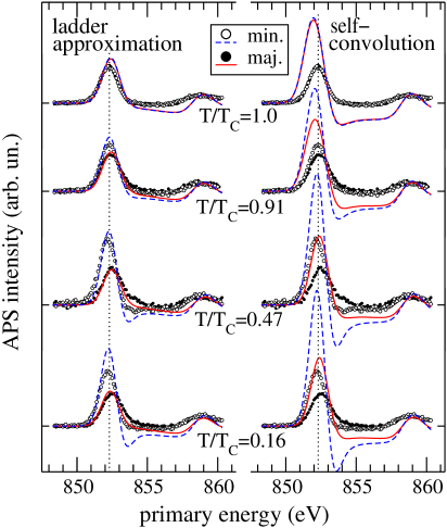
Figure 2: (from Ref. PWN+00 ) Spin-resolved $L_{\rm III}$ Ni AP spectrum for different reduced temperatures $T/T_{\rm C}$. Data points: measured differential intensity $dI/dE$ as a function of the primary energy. For better comparison with theory the same data are shown twice (left and right panel). Lines, left: theory with direct and indirect correlations included (ladder approximation). Lines, right: indirect correlations included only (self-convolution)

Hamiltonian.

To study the significance of electron correlations, we consider a nine-band Hubbard-type model $H=H_{0}+H_{1}$ including correlated $3d$ and uncorrelated $4s$/$4p$ orbitals as given by Eq. (25). The first (“free”) term $H_{0}$ is obtained from a Slater-Koster fit to the paramagnetic LDA band structure for Ni WPN00 . Opposed to PES/IPE, this comparatively simple tight-binding parameterization appears to be sufficient in the case of APS since the two-particle spectrum does not crucially depend on the details of the one-particle DOS.

The on-site interaction among the $3d$ electrons is described by the second term $H_{1}$. Exploiting atomic symmetries the Coulomb-interaction parameters which depend on the four orbital indices $m_{1},\ldots,m_{4}$ can essentially be expressed in terms of two independent parameters $U$ and $J$. The numerical values for the direct and exchange interaction, $U=2.47$ eV and $J=0.5$ eV, are taken from Ref. WPN00 where they have been fitted to the ground-state magnetic properties of Ni. Residual interactions involving de-localized $s$ and $p$ states are assumed to be sufficiently accounted for by the LDA. Finally, a double-counting correction is applied to $H$ since partially the interaction $H_{1}$ is already included in the LDA Hamiltonian $H_{0}$ (for details see Ref. WPN00 ).

Green functions.

The two-particle Green function in Eq. (27) is approximately calculated by using standard diagrammatic techniques. Because of the low density of $3d$ holes in the case of Ni, it appears to be reasonable to employ the so-called ladder approximation Nol90 which extrapolates from the exact (Cini-Sawatzky) solution for the limit of the completely filled valence band Cin77 ; Saw77 . For finite hole densities the ladder approximation gives the two-particle as a functional $\cal F$ of the one-particle Green function (direct correlations).

The one-particle Green function, which describes the indirect correlations, is calculated self-consistently within second-order perturbation theory (SOPT) around the Hartree-Fock solution WPN00 . For a moderate $U$ and a low hole density, a perturbational approach can be justified SAS92 . A re-summation of higher-order diagrams is important to describe bound states (“Ni 6 eV satellite”) Lie81 which, however, are relevant for AES only. Since spin-wave excitations are neglected in the approach, the calculated Curie temperature $T_{\rm C}=1655$ K is about a factor 2.6 too high. Using reduced temperatures $T/T_{\rm C}$, however, the temperature trend of the magnetization is well reproduced WPN00 .

Matrix elements.

The transition-matrix elements in Eq. (27),

$$M_{L_{1}L_{2}}^{\sigma_{c}\sigma_{i}}({\bf k}_{\|},E)=\langle\mbox{2p},\sigma_{c}|\>\langle{\bf k}_{\|}E\sigma_{i}|\>r_{12}^{-1}\>|iL_{1}\sigma_{c}\rangle\>|iL_{2}\sigma_{i}\rangle\>,$$ (28)

are calculated by assuming the transition to be intra-atomic as usual Ram91 ; HWMR88 ; EP97 . The different wave functions as well as the Coulomb operator $1/r_{12}$ are expanded into spherical harmonics, the angular integrations are performed analytically, and the numerical radial integrations are cut at the Wigner-Seitz radius.

Surface effects enter the theory via the high-energy scattering state $|{\bf k}_{\|}E\sigma_{i}\rangle$. It is calculated as a conventional LEED state with ${\bf k}_{\|}=0$ to describe the normally incident electron beam in the experimental setup. The (paramagnetic) LDA potential for Ni is determined by a self-consistent tight-binding linear muffin-tin orbitals (LMTO) calculation AJ84 . The $3d$, $4s$, and $4p$ valence orbitals $|iL\sigma\rangle$ are taken to be the muffin-tin orbitals. The four-fold degenerate $2p_{3/2}$ core state is obtained from the LDA core potential by solving the radial Dirac equation numerically. Its (relativistically) large component is decomposed into a (coherent) sum of Pauli spinors $|\mbox{2p},\sigma_{c}\rangle$ with $\sigma_{c}=\uparrow,\downarrow$.

Results.

The solid lines in Fig. 2 (left) show the spectra as calculated from Eq. (27) using the ladder approximation for the two-particle Green function. To account for apparatus broadening, the results have been folded with a Gaussian of width $\sigma=0.6$ eV (see Ref. EP97 ). The calculated data are shifted by 852.3 eV such that onset of the un-broadened spectrum for $T/T_{\rm C}=0.16$ coincides with the maximum of $L_{\rm III}$ emission in the experiment (dotted line). Fig. 2 and also a more detailed inspection show that the secondary peak at $E\approx 859$ eV is not affected by correlations at all. This is consistent with observed temperature independence of the peak and with the fact that the DOS has mainly $s$-$p$ character at the discontinuity deriving from the $L_{7}$ critical point. The maximum of the secondary peak is therefore used as a reference to normalize the measured spectra for each temperature.

What are the signatures of electron correlations? The indirect correlations manifest themselves as a renormalization of the one-particle DOS. Here, they are responsible in first place for the correct temperature dependence of the intensity asymmetry of the main peak in the AP spectrum. Details are discussed in Refs. WPN00 ; PWN+00 . The the direct interaction between the two additional final-state electrons and thus the direct correlations are much more important for APS. To estimate this effect, Fig. 2 (right) also displays the results of the self-convolution model for comparison (still including matrix elements as well as the fully interacting one-particle DOS).

Looking at the results of the ladder approximation, the overall agreement with the measurements is rather satisfying. Except for the lowest temperature the intensity, the spin splitting and the spin asymmetry of the main peak are well reproduced and, consistent with the experiment, a negligibly small intensity asymmetry and spin splitting is predicted for the secondary peak. However, switching off the direct correlations (Fig. 2, right), results in a strong overestimation of the main peak structure.

A plausible qualitative explanation of this pronounced correlation effect can given within the Cini-Sawatzky theory: For low hole density the main effect of the direct correlations is known to transfer spectral weight to lower energies inaccessible to APS. This weight shows up again in the (complementary) Auger spectrum (recall that APS and AES are described by the same Green function). Hypothetically, for $U\mapsto\infty$ all weight would be taken by a satellite split off at the lower boundary of the Auger spectrum Cin77 ; Saw77 . A considerable weight transfer is in fact seen in AES Ram91 ; BFHLS83 .

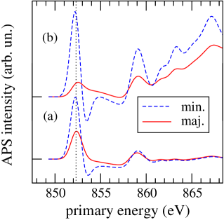
Figure 3: (from Ref. PWN+00 ) Ni AP spectrum for $T=0$. (a) full theory. (b) as (a) but matrix elements taken to be constant (see text)

Fig. 3 shows the effect of the transition-matrix elements. Their importance for a quantitative understanding of spin-resolved APS can be demonstrated by setting $M_{L_{1}L_{2}}^{\sigma_{c}\sigma_{i}}({\bf k}_{\|},E)=\pm 1=\mbox{const}$ for $L_{1}\geq L_{2}$ or $L_{1}<L_{2}$, respectively, (see below) and comparing with the results of the full theory. Their energy dependence (via the energy dependence of $|{\bf k}_{\|}E\sigma_{i}\rangle$) is weak over a few eV at energies of the order of keV and cannot explain the difference between (a) and (b) in Fig. 3. The main difference is rather a consequence of the fact that the radial $2p$ core wave function has a stronger overlap with the (more localized) $3d$ as compared to the (more de-localized) $4s/4p$ radial wave functions. This implies a suppression of the $s$-$p$ contributions to the orbital sum in Eq. (27). The features above $E=860$ eV originate from additional discontinuities of the $s$-$p$-like DOS (as for the peak at $E\approx 859$ eV).

For $T<T_{\rm C}$ the spin asymmetry of the spectrum is mainly due to the spin dependence of the Green function in Eq. (27). If the calculation of the matrix elements (28) starts from the spin-polarized L(S)DA potential, an additional spin asymmetry is observed resulting from the spin dependence of the states in Eq. (28). This, however, is small and has practically no influence on the results.

On the other hand, Fig. 3 shows a strong suppression of the intensity asymmetry at high energies when taking matrix elements into account. This effect is controlled by the symmetry of the matrix $M_{L_{1}L_{2}}\equiv M_{L_{1}L_{2}}^{\sigma_{c}\sigma_{i}}({\bf k}_{\|},E)$. In the antisymmetric case, $M_{L_{1}L_{2}}=-M_{L_{2}L_{1}}$ ($L_{1}\neq L_{2}$), there is a maximum spin asymmetry (Fig. 3) while, even for a ferromagnet, there is no spin asymmetry at all for the symmetric case, as discussed in section 3. The results of the full calculation along Eq. (28) are neither fully symmetric nor antisymmetric with respect to $L_{1}$, $L_{2}$.

5 Conclusions

It has been shown that the basic theory of different electron spectroscopies, PES, IPE, AES and APS, can be developed within a unified framework. Starting from Fermi’s golden rule and employing the sudden approximation, the intensity can be expressed in terms of a one- or two-particle Green function including electron-photon or Coulomb matrix elements, respectively. Citing APS from the typical band ferromagnet Ni as an example, it could be demonstrated that a quantitative agreement with spin-resolved and temperature-dependent measured spectra can be achieved when the basic spectroscopic formula is taken seriously and is evaluated by modern techniques of solid-state theory.

In particular, it has been demonstrated that there are pronounced (direct) correlation effects in the AP line shape of Ni. While $s$-$p$ derived features at higher energies appear to be sensitive to the geometrical structure only, the main peak is strongly affected by the direct interaction between the two additional final-state electrons. Consistent with the Cini-Sawatzky model and consistent with the well-known Ni Auger spectrum, there is a considerable spectral-weight transfer to energies below the threshold. For Co and Fe one can even expect stronger effects of $d$-$d$ correlations on the AP line shape since the $d$-hole density is larger than in Ni. Simple self-convolution models neglecting the direct correlations must be questioned seriously.

It has also been demonstrated that a mere computation of the (two-particle) Green function is insufficient to describe spin-resolved APS. The spin asymmetry of the AP signal is found to be mainly determined by the orbital-dependent transition-matrix elements and their transformation behavior under exchange of the orbital quantum numbers.

Considering the temperature dependence of the spectra and the magnetic order resulting from strong (indirect) correlations in addition, one can state that the AP line shape of a typical ferromagnetic $3d$ transition metal is determined by a rather complex interplay of different factors.

Despite the fact that a reasonable understanding of APS from Ni has been achieved, there is much work to be done in the future: An open question concerns the importance of core-hole effects in APS, for example. For the present case there has been no need to consider scattering at the core-hole potential in the final state. This may likely be different for systems with a smaller $3d$ occupancy. Furthermore, one must recognize that even the determination of the valence-band Green function is a central problem of many-body theory. Recently much progress has been achieved to deal with single-band models GKKR96 ; for a quantitative interpretation of electron spectra from transition metals, however, one needs a theory that realistically includes orbital degeneracy and $sp$-$d$ hybridization from the very beginning. Compared to perturbation theory or lowest-order re-summation of diagrams, as employed here, improvements are conceivable and necessary albeit not easily performed.

Acknowlegdements

I would like to thank J. Braun, M. Donath (Universität Münster), W. Nolting, T. Wegner (Humboldt-Universität zu Berlin) and T. Schlathölter (Philips Hamburg) for stimulating discussions.

References

- (1) J. B. Pendry: Low Energy Electron Diffraction (Academic, London 1974)
- (2) R. L. Park, J. E. Houston: J. Vac. Sci. Technol. 11, 1 (1974)
- (3) Photoemission and the Electronic Properties of Surfaces, ed. by B. Feuerbacher, B. Fitton, R. F. Willis (Wiley, New York 1978)
- (4) J. C. Fuggle: Electron Spectroscopy: Theory, Techniques and Applications, vol. 4 (Academic, London 1981) p. 85
- (5) D. E. Ramaker: Crit. Rev. Solid State Mater. 17, 211 (1991)
- (6) M. Donath: Surf. Sci. Rep. 20, 251 (1994)
- (7) J. B. Pendry: Surf. Sci. 57, 679 (1976)
- (8) G. Borstel: Appl. Phys. A 38, 193 (1985)
- (9) J. Braun: Rep. Prog. Phys. 59, 1267 (1996)
- (10) P. Hohenberg, W. Kohn: Phys. Rev. 136, 864 (1964)
- (11) W. Kohn, L. J. Sham: Phys. Rev. 140, 1133 (1965)
- (12) M. Potthoff, J. Lachnitt, W. Nolting, J. Braun: phys. stat. sol. (b) 203, 441 (1997)
- (13) C. Meyer, M. Potthoff, W. Nolting, G. Borstel, J. Braun: phys. stat. sol. (b) 216, 1023 (1999)
- (14) J. J. Lander: Phys. Rev. 91, 1382 (1953)
- (15) G. Hörmandinger, P. Weinberger, P. Marksteiner, J. Redinger: Phys. Rev. B 38, 1040 (1988)
- (16) H. Ebert, V. Popescu: Phys. Rev. B 56, 12884 (1997)
- (17) J. Kirschner: Solid State Commun. 49, 39 (1984)
- (18) K. Ertl, M. Vonbank, V. Dose, J. Noffke: Solid State Commun. 88, 557 (1993)
- (19) M. Cini: Solid State Commun. 24, 681 (1977)
- (20) G. A. Sawatzky: Phys. Rev. Lett. 39, 504 (1977)
- (21) A. A. Abrikosow, L. P. Gorkov, I. E. Dzyaloshinski: Methods of Quantum Field Theory in Statistical Physics (Prentice-Hall, New Jersey 1964).
- (22) M. Potthoff, J. Braun, W. Nolting, G. Borstel: J. Phys.: Condens. Matter 5, 6879 (1993)
- (23) M. Potthoff, J. Braun, G. Borstel: Z. Phys. B 95, 207 (1994)
- (24) M. Vonbank: Spinaufgelöste Appearance Potential Spektroskopie an 3d-Übergangsmetallen. PhD Thesis, TU Wien (1992)
- (25) M. Potthoff, T. Wegner, W. Nolting, T. Schlathölter, M. Vonbank, K. Ertl, J. Braun, M. Donath (to be published)
- (26) T. Wegner, M. Potthoff, W. Nolting: Phys. Rev. B 61, 1386 (2000)
- (27) W. Nolting: Z. Phys. B 80, 73 (1990)
- (28) M. M. Steiner, R. C. Albers, L. J. Sham: Phys. Rev. B 45, 13272 (1992)
- (29) A. Liebsch: Phys. Rev. B 23, 5203 (1981)
- (30) O.K. Andersen, O. Jepsen: Phys. Rev. Lett. 53, 2571 (1984)
- (31) P. A. Bennett, J. C. Fuggle, F. U. Hillebrecht, A. Lenselink, G. A. Sawatzky: Phys. Rev. B 27, 2194 (1983)
- (32) A. Georges, G. Kotliar, W. Krauth, M. J. Rozenberg: Rev. Mod. Phys. 68, 13 (1996)