Magnetic exchange interaction induced by a Josephson current

I Introduction

Despite their apparent simplicity, ferromagnet–normal-metal–ferromagnet trilayers exhibit many interesting properties. One example is the equilibrium exchange interaction between the magnetic moments of the two ferromagnets, which is mediated by the coherent electron motion in the normal metal spacer layer.[1] Depending on the thickness of the spacer layer, this interaction may favor parallel or antiparallel alignment of the magnetic moments,[1, 2] or, in some cases, even perpendicular alignment.[3, 4] In addition, a torque may be exerted on the magnetic moments when an electrical current is passed through the trilayer. For this nonequilibrium magnetic torque, the preferred magnetic configuration (parallel or antiparallel) was found to depend on the sign of the current,[5, 6, 7, 8] so that a reversal of the current switches the magnetic moment of the ferromagnets from parallel to anti-parallel. This reversal can be observed by a measurement of the conductance, which is larger in the parallel configuration than in the antiparallel one (this is known as giant magneto resistance[9]).

A unified description of equilibrium and nonequilibrium torques can be given using the concept of spin current. In the case of a ferromagnet–normal-metal–ferromagnet (FNF) trilayer, this description was introduced by Slonczewski as an alternative way to calculate the equilibrium exchange interaction.[10] (The “standard” way to calculate the exchange interaction involves a computation of the derivative of the free energy to the angle between the two magnetic moments.) When electrons scatter from a spin-dependent potential, as is appropriate for a mean-field description of ferromagnetism, the spin current carried by the conduction electrons need not be conserved. Since the total spin of the system (i.e., the combined moment of the conduction electrons and the other electrons responsible for the magnetic moment in the ferromagnetic layers) is conserved, the lost spin current must have been transferred to the magnetic moment of the ferromagnet, which means that a torque is exerted on the moments of the ferromagnets. In this way, the equilibrium exchange interaction is seen to follow from an equilibrium spin current flowing from one ferromagnet to the other,[10] much like the equilibrium (persistent) current that exist in mesoscopic metal rings,[11] whereas the nonequilibrium torque arises from the non-conservation of spin currents flowing in conjunction with the electrical current.[5]

The nonequilibrium torque is changed when the FNF trilayer is coupled to one superconductor (S) contact and one normal-metal (N) contact, instead of to two normal-metal contacts. The main difference between N and S contacts is that the former can carry both spin and charge currents, while the latter can only carry a charge current for voltages below the superconducting gap $\Delta_{0}$. In a previous publication, we showed that this restriction gives rise to a nonequilibrium torque that, depending on the direction of the electrical current, can lead to the switching of the magnetic moments to a perpendicular configuration, rather than a parallel or antiparallel one.[12] The equilibrium torque (i.e., the magnetic exchange interaction), however, is not qualitatively affected by the presence of the one superconducting contact.[13]

In this paper, we consider an FNF junction with two superconducting contacts. For this system, a macroscopic supercurrent may flow through the junction already in equilibrium, the magnitude and sign of the current depending on the phases of the order parameters of the two superconductors. As ferromagnets break time-reversal symmetry, they are expected to suppress the Josephson effect. However for sufficiently thin or weak ferromagnetic layers (for instance a Cu_1-xNi_x alloy [14] with $x>0.44$) , the Josephson effect may survive. Magnetic Josephson junctions with one ferromagnetic layer have received considerable attention because of the possibility of $\pi$-junction behavior,[15, 16, 17, 18] which has been observed experimentally only recently.[14, 19] Josephson junctions with two magnetic layers were studied in Refs. [20, 21], where it was shown that the supercurrent for antiparallel alignment of the magnetic moments can be larger than for parallel alignment.

Here, we consider the exchange interaction in an FNF junction with two superconducting contacts. We find that the equilibrium exchange interaction is deeply affected by the presence of the superconductors. By the same mechanism by which the supercurrent depends on the relative orientation of the two magnetic moments,[20, 21] the exchange interaction depends on the phase difference between the two superconducting order parameters. As a result, the supercurrent controls the exchange interaction between the two magnetic moments. In contrast to the usual magnetic exchange interaction, which involves contributions from the whole energy band, the Josephson current induced magnetic exchange interaction is carried only by states with an energy within a distance of order $\Delta_{0}$ from the Fermi energy. At a first glance, one is tempted to consider the Josephson current induced torque as the direct analogue of the nonequilibrium current-induced torque that exists for normal metal contacts. However, as we’ll show in the remainder of this paper, that is not the case: Apart from its magnitude, the Josephson current induced torque has most of the features of the standard equilibrium magnetic exchange interaction.

This article is devoted to the study of the Josephson current induced magnetic exchange interaction and to its consequences on the dynamics of the magnetic moments. It is organized as follows: In Section II, we present the concept of spin current and discuss the differences between equilibrium and nonequilibrium torque. We then focus on the case of a Josephson junction (both electrodes superconducting). Section III contains a brief review of the scattering approach, that allows for practical calculation of the torques discussed in Section II. We are then ready to discuss, in Section IV, the magnetic exchange interaction in the Josephson junction, using various models for the scattering matrices of the normal and ferromagnetic layers involved. Finally, the effect of the torque on the dynamics of the magnetic moments is briefly discussed in Section V.

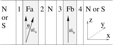
FIG. 1.: Schematic of the trilayer system considered in this article. $F_{a}$ and $F_{b}$ are the ferromagnetic layers and $\vec{m}_{a}$ and $\vec{m}_{b}$ their respective magnetic moments. The ferromagnetic layers are separated by a normal spacer $N$ and are connected to two reservoirs that can be either normal ($N$) or superconducting ($S$). The numbers $1$, $2$, $3$, $4$ stand for ideal fictitious leads that have been added for technical convenience.

II Spin current and spin torque

The system we consider is shown in Fig. 1. It consists of a ferromagnet–normal-metal–ferromagnet trilayer, connected to (possibly superconducting) electrodes on the right and the left. The two ferromagnetic layers are labeled $F_{a}$ and $F_{b}$, the normal metal spacer layer is labeled $N$. The magnetic moments of $F_{a}$ and $F_{b}$ point in the direction of unit vectors $\hat{m}_{a}$ and $\hat{m}_{b}$, respectively. The angle between $\hat{m}_{a}$ and $\hat{m}_{b}$ is $\theta$. We assume that $\hat{m}_{b}$ points in the $z$-direction. For technical convenience, we have added pieces of ideal lead (labeled $1$, $2$, $3$, and $4$) between the layers $F_{a}$, $N$, and $F_{b}$, and the reservoirs.

The conduction electrons are described by an effective Hamiltonian,[22]

$$H_{\rm eff} = \int d\vec{r}\sum_{\alpha,\beta=\uparrow,\downarrow}\Psi^{\dagger}_{\alpha}(\vec{r})H_{\alpha\beta}\Psi_{\beta}(\vec{r})$$ (2)

$$\mbox{}+\int d\vec{r}\left[\Delta(\vec{r})\Psi^{\dagger}_{\uparrow}(\vec{r})\Psi^{\dagger}_{\downarrow}(\vec{r})+\Delta^{*}(\vec{r})\Psi_{\downarrow}(\vec{r})\Psi_{\uparrow}(\vec{r})\right],$$

where $\Psi^{\dagger}_{\alpha}(\vec{r})$ creates an electron with spin $\alpha$ and $\Delta(\vec{r})$ is the superconducting gap. In the normal regions, $\Delta(\vec{r})=0$. Finally, the $2\times 2$ matrix

$$H=-(\hbar^{2}/2m)\nabla^{2}+V(\vec{r})-E_{F}$$

contains kinetic, potential, and Fermi energy. The potential $V(\vec{r})$ represents the spin-independent scattering from impurities, as well as the spin-dependent effect of the local exchange field inside the ferromagnets. For simplicity, we assume that the local exchange field is always parallel to the total magnetization of the layer (which corresponds to the neglect of spin-flip scattering). Thus we have

$$V(\vec{r})=e^{-i\frac{\sigma_{y}\theta(\vec{r})}{2}}\left(\begin{array}[]{cc}V_{\rm maj}(\vec{r})&0\\ 0&V_{\rm min}(\vec{r})\end{array}\right)e^{i\frac{\sigma_{y}\theta(\vec{r})}{2}}.$$ (3)

Here, maj (min) stands for majority (minority) and $\exp[-i\sigma_{y}\theta(\vec{r})/2]$ is a rotation matrix rotating from the external reference frame to the direction of the local exchange field. Outside the ferromagnets, $V_{\rm maj}=V_{\rm min}$. For the system under consideration, the angle $\theta(\vec{r})=\theta$ inside $F_{a}$ and zero elsewhere.

An expression for the spin current is obtained by writing down the conservation equation for the spin density $\vec{\eta}(\vec{r})$,

$$\vec{\eta}(\vec{r})=\frac{\hbar}{2}\sum_{\alpha\beta}\Psi^{\dagger}_{\alpha}(\vec{r})\vec{\sigma}_{\alpha\beta}\Psi_{\beta}(\vec{r}),$$ (4)

$\vec{\sigma}=(\sigma_{x},\sigma_{y},\sigma_{z})^{T}$ being the vector of pauli matrices. The time evolution of spin density reads,

$$\frac{\partial}{\partial t}\langle\vec{\eta}(\vec{r})\rangle = \frac{i}{\hbar}\langle[H_{\rm eff},\vec{\eta}(\vec{r})]\rangle$$ (5)

$$= -\vec{\nabla}\cdot\stackrel{{\scriptstyle\Rightarrow}}{{j}}(\vec{r})+\frac{i}{2}\langle\Psi^{\dagger}(\vec{r})[V(\vec{r}),\vec{\sigma}]\Psi(\vec{r})\rangle,$$ (6)

with the spin current density tensor $\stackrel{{\scriptstyle\Rightarrow}}{{j}}$ defined as,

$$\stackrel{{\scriptstyle\Rightarrow}}{{j}}(\vec{r})=-\frac{i\hbar^{2}}{4m}\langle\Psi^{\dagger}(\vec{r})\vec{\nabla}\vec{\sigma}\Psi(\vec{r})-\vec{\nabla}\Psi^{\dagger}(\vec{r})\vec{\sigma}\Psi(\vec{r})\rangle.$$ (7)

The spin current density has one index in spin space and one in real space while the brackets $\langle\ldots\rangle$ stands for the quantum mechanical expectation value. Equation (5) shows that, unlike charge current, spin current is not conserved inside the ferromagnets. In fact, the current induced torque and the magnetic exchange interaction follow from the spin current lost by the conduction electrons inside the ferromagnets. The current induced torque follows from the non-conservaton of non-equilibrium spin current, while the magnetic exchange interaction follows from the non-conservation of the equilibrium spin current between $F_{a}$ and $F_{b}$. The total torque $\vec{\tau}_{a}$, $\vec{\tau}_{b}$ (i.e., the sum of equilibrium and non-equilibrium contributions) on the layers $F_{a}$ and $F_{b}$ is found as

$$\vec{\tau}_{a}=\vec{J}_{1}-\vec{J}_{2}\ \ ,\ \ \vec{\tau}_{b}=\vec{J}_{3}-\vec{J}_{4},$$ (8)

where $\vec{J}_{i}$ is the total spin current that flows in the $x$ direction in region $i$ ($i=1,2,3,4$),

$$\vec{J}_{i}=\int dydz\ \vec{j}_{x}(x,y,z),\ \ \ x\in i.$$ (9)

We now focus on the torque $\vec{\tau}_{a}$ on the magnetic moment of layer $F_{a}$. In addition to the unit vector $\hat{m}_{a}$ that points along the magnetization direction of $F_{a}$, we introduce the unit vectors $\hat{v}=\hat{m}_{a}\times\hat{m}_{b}/|\hat{m}_{a}\times\hat{m}_{b}|$, which points normal to the plane spanned by $\hat{m}_{a}$ and $\hat{m}_{b}$, and $\hat{w}=\hat{m}_{a}\times\hat{v}$, which lies in the plane spanned by $\hat{m}_{a}$ and $\hat{m}_{b}$, but points perpendicular to $\hat{m}_{a}$, see Fig. 2. For the configuration of Fig. 1, $\hat{v}$ is the unit vector in the $y$ direction and the plane spanned by $\hat{m}_{a}$ and $\hat{m}_{b}$ is the $xz$ plane. From the observation that

$$\left[V(\vec{r}),\sigma_{y}\right]=-2i\frac{\partial V}{\partial\theta},$$ (10)

combined with Eq. (5), we find that the out-of-plane component of the torque $\tau_{a}^{v}=\vec{\tau}_{a}\cdot\hat{v}$ is equal to the derivative of the energy $E=\langle H\rangle$ of the trilayer to the angle $\theta$. No such simple result can be found for the torque in the $\hat{w}$-direction (the component of the torque in the plane spanned by $\hat{m}_{a}$ and $\hat{m}_{b}$). Hence, we find for the total torque acting on the magnetic moment of $F_{a}$

$$\vec{\tau}_{a} = \tau_{a}^{v}\hat{v}+\tau_{a}^{w}\hat{w},$$ (12)

$$\tau_{a}^{v} = \frac{\partial E}{\partial\theta},$$ (13)

$$\tau_{a}^{w} = -\frac{1}{2}\int_{\vec{r}\in F_{a}}d\vec{r}\,\langle\Psi^{\dagger}(\vec{r})(V_{\rm maj}-V_{\rm min})(\vec{\sigma}\cdot\hat{v})\Psi(\vec{r})\rangle.$$ (14)

Since the spin current in the direction of $\hat{m}_{a}$ is always conserved in the absence of spin-flip scattering, there is no component of the torque along $\hat{m}_{a}$, cf. Eq. (5). Although the above derivation may seem a little specific, Eq. (10) can be shown to hold as well in the presence of two-body interactions.

FIG. 2.: Schematic of the out of plane component of the torque $\tau_{a}^{v}\hat{v}$ (left side) and the in-plane component of the torque $\tau_{a}^{w}\hat{w}$ (right side). The equilibrium exchange interaction only has an out of plane component while the non equilibrium torque is mainly in plane.

As seen from Eq. (10), the total torque consists of two contributions, which are sketched in Fig. 2. The in-plane torque $\tau^{w}_{a}$ directly pushes $\hat{m}_{a}$ towards or away from $\hat{m}_{b}$. It is the main component of the nonequilibrium torque, which is discussed in Refs. [5, 8]. In equilibrium, however, no spin current can flow outside the trilayer, so that, by Eq. (8),

$$\vec{\tau}_{a}^{\rm equ}=-\vec{J}_{2}=-\vec{J}_{3}=-\vec{\tau}_{b}^{\rm equ}.$$ (15)

Combined with the requirement that $\vec{\tau}_{a}$ ($\vec{\tau}_{b}$) is perpendicular to $\hat{m}_{a}$ ($\hat{m}_{b}$), this relation implies that, in equilibrium, the in-plane torque $\tau_{a}^{w}$ vanishes.[13] The out-of-plane torque $\tau_{a}^{v}$ causes a precession of one magnetic moment around the other one. This is similar to the Larmor precession of the moments in a (possibly $\theta$-dependent) magnetic field. In the presence of dissipation, the system will then relax to the lowest energy configuration, where the energy is minimal and, hence, by Eq. (13), the torque zero.

According to Eqs. (15) and (13), there are two, equivalent, ways to calculate the equilibrium torque $\vec{\tau}_{a}^{\rm equ}$: As the equilibrium spin current $\vec{J}_{2}$ flowing from $F_{a}$ to $F_{b}$, or as the derivative of the ground state energy $E$ to the angle $\theta$ between $\hat{m}_{a}$ and $\hat{m}_{b}$. (Note that there is a direct analogy between the equilibrium spin current flowing inside the trilayer with an angle $\theta$ between the two magnetic moments and the persistent current in a mesoscopic ring in presence of an Aharonov-Bohm flux.) In the remainder of this paper, we concentrate on the equilibrium torque in the case where both left and right electrodes are superconducting.

The effective Hamiltonian $H_{\rm eff}$ can be diagonalized by the Bogoliubov transformation,

$$\Psi_{\alpha}(\vec{r})=\sum_{\epsilon>0}u_{\alpha,\epsilon}(\vec{r})\gamma_{\epsilon}+v^{*}_{\alpha,\epsilon}(\vec{r})\gamma^{\dagger}_{\epsilon},$$ (16)

where the fermion operator $\gamma^{\dagger}_{\epsilon}$ creates an excitation at energy $\epsilon$ and $u$ ($v$) is the electron (hole) component of the solution to the Bogoliubov-De Gennes equation at energy $\varepsilon$,[22]

$$\left(\begin{array}[]{cc}H&i\Delta\sigma_{y}\\ -i\Delta^{*}\sigma_{y}&-H^{*}\end{array}\right)\left(\begin{array}[]{c}u\\ v\end{array}\right)=\epsilon\left(\begin{array}[]{c}u\\ v\end{array}\right).$$ (17)

In principle, the superconducting order parameter $\Delta(\vec{r})$ has to be calculated self-consistently,

$$\Delta(\vec{r})=-\frac{i}{2}|g(\vec{r})|\sum_{\epsilon>0}[1-2f(\epsilon)]\ v^{\dagger}\sigma_{y}u,$$ (18)

where $g(\vec{r})$ is the BCS interaction constant, which is finite inside the superconductor and drops abruptly to zero outside S, and $f(\epsilon)$ is the Fermi function. Here, we adopt the simple model that $\Delta(\vec{r})$ has its bulk value $\Delta=\Delta_{0}e^{i\phi/2}$ ($\Delta=\Delta_{0}e^{-i\phi/2}$) inside the left (right) superconducting reservoirs, while $\Delta=0$ in the normal layers. At the normal-metal–superconductor interface, $\Delta(\vec{r})$ can be approximated by a step function. This approximation, discussed in Ref. [23], is valid for the quasi-one dimensional geometry we consider here. Up to terms that are independent of $\theta$ and $\phi$, $H_{\rm eff}$ reads

$$H_{\rm eff}=-\frac{1}{2}\sum_{\epsilon>0}\epsilon+\sum_{\epsilon>0}\epsilon\ \gamma^{\dagger}_{\epsilon}\gamma_{\epsilon}.$$ (19)

Combining Eqs. (7) and (16), one obtains for the spin current

$$\stackrel{{\scriptstyle\Rightarrow}}{{j}}=\frac{\hbar^{2}}{2m}{\rm Im}\sum_{\epsilon>0}\left(u^{\dagger}\vec{\nabla}\vec{\sigma}u-v^{T}\vec{\nabla}\vec{\sigma}v^{*}\right)\langle\gamma_{\epsilon}^{\dagger}\gamma_{\epsilon}-\frac{1}{2}\rangle.$$ (20)

Equation (20) was used to calculate the non-equilibrium torque for an FNF trilayer with one superconducting contact in Ref. [12]. In that case, only eigenstates of the Bogoliubov-de Gennes equation with energy close to the Fermi level were involved, so that an analog of the Landauer formula could be derived to find the nonequilibrium current-induced torque. The equilibrium torque, however, is of a very different nature since it involves all states in the entire conduction band. This limits theoretical approaches to analytical calculations for simple model systems [1] or ab-initio numerical simulations.[2] This difficulty does not occur for the Josephson current induced torque.

In a Josephson junction, the equilibrium current $I$ at finite temperature is given by the derivative of the free energy $F$ of the junction to the phase difference $\phi$ between the two superconductors,[22]

$$I=\frac{2e}{\hbar}\frac{\partial F}{\partial\phi}.$$ (21)

This equation is very similar to the equation for the equilibrium spin current between the two ferromagnetic layers, $J_{2}=-\tau_{a}^{\rm equ}$, where Eq. (10) gives

$$\tau_{a}^{\rm equ}=\frac{\partial F}{\partial\theta}.$$ (22)

Combining these last two equations one finds that,

$$\frac{\partial I}{\partial\theta}=\frac{2e}{\hbar}\frac{\partial\tau_{a}^{\rm equ}}{\partial\phi}.$$ (23)

In other words, a $\theta$-dependence of the supercurrent implies a $\phi$-dependence of the equilibrium torque. This is a very suggestive result, as it was recently predicted that the Josephson current should be very sensitive to the angle $\theta$ between the two magnetic moments.[20, 21] In what follows, we refrain from calculating the full equilibrium torque but concentrate on it $\phi$-dependent part, the rationale being that it is precisely the $\phi$-dependent part that can be viewed as the supercurrent induced torque. As we shall see, the $\phi$-dependent part of the torque only has contributions from energies within $\Delta_{0}$ of the Fermi energy and can, therefore, be calculated from the scattering properties of the junction at and near the Fermi level.

III Scattering matrix formalism

A general review of the scattering matrix formalism can be found in Ref. [25], while the particular application to the calculation of spin currents in FNF trilayers is discussed in Ref. [8]. Below we give a brief compilation of the necessary formulas for the calculation of the equilibrium torque in an FNF trilayer with two superconducting contacts.

The trilayer is bounded in the $y$ and $z$ directions, so that the corresponding degrees of freedom are quantized and give rise to $N_{\rm ch}$ propagating modes at the Fermi level, with $N_{\rm ch}\sim A/\lambda_{F}^{2}$, $A$ being the cross section of the junction and $\lambda_{F}$ the Fermi wave length. Each transverse mode appears as a left moving mode and as a right moving mode, and with components for particle/hole and spin degrees of freedom. We expand the solution of the BdG equation in terms of these modes and describe wavefunctions in terms of the $4N_{\rm ch}$-component vectors $\Psi_{i}^{L(R)}$ which are the projection of the wave functions $(u,v)$ on the left (right) going modes in the ideal lead $i$ ($i=1,2,3,4$, see Fig. 1). The layers $F_{a}$, $F_{b}$, and $N$ are characterized by $8N_{\rm ch}\times 8N_{\rm ch}$ unitary scatterings matrices ${\cal S}_{a}$, ${\cal S}_{b}$, and ${\cal S}_{N}$, respectively,

$$\left(\begin{array}[]{c}\Psi_{1}^{L}\\ \Psi_{2}^{R}\end{array}\right) = {\cal S}_{a}\left(\begin{array}[]{c}\Psi_{1}^{R}\\ \Psi_{2}^{L}\end{array}\right),$$ (28)

$$\left(\begin{array}[]{c}\Psi_{2}^{L}\\ \Psi_{3}^{R}\end{array}\right) = {\cal S}_{N}\left(\begin{array}[]{c}\Psi_{2}^{R}\\ \Psi_{3}^{L}\end{array}\right),$$ (33)

$$\left(\begin{array}[]{c}\Psi_{3}^{L}\\ \Psi_{4}^{R}\end{array}\right) = {\cal S}_{b}\left(\begin{array}[]{c}\Psi_{3}^{R}\\ \Psi_{4}^{L}\end{array}\right).$$ (38)

Each of the matrices ${\cal S}_{i}$ ($i=a,b,N$) is further decomposed into $4N_{\rm ch}\times 4N_{\rm ch}$ reflection ($r_{i}$, $r^{\prime}_{i}$) and transmission ($t_{i}$, $t^{\prime}_{i}$) matrices,

$${\cal S}_{i}=\left(\begin{array}[]{cc}r_{i}&t^{\prime}_{i}\\ t_{i}&r^{\prime}_{i}\end{array}\right).$$ (39)

Further, the scattering matrices ${\cal S}_{i}$ are diagonal in electron-hole space,

$${\cal S}_{i}(\epsilon)=\left(\begin{array}[]{cc}{S}_{i}(\epsilon)&0\\ 0&{S}^{*}_{i}(-\epsilon)\\ \end{array}\right),$$ (40)

whereas, in spin space, ${\cal S}_{N}$ is proportional to the $2\times 2$ identity matrix, ${\cal S}_{b}={\rm diag}(S_{b\uparrow},S_{b\downarrow})$ is diagonal, and ${\cal S}_{a}$ reads

$${\cal S}_{a}=e^{-i\frac{\sigma_{y}\theta}{2}}\left(\begin{array}[]{cc}S_{a\uparrow}&0\\ 0&S_{a\downarrow}\end{array}\right)e^{i\frac{\sigma_{y}\theta}{2}}.$$ (41)

Finally, the full scattering matrix ${\cal S}_{\vphantom{FNF}}$ of the trilayer can be calculated by combining ${\cal S}_{a}$, ${\cal S}_{N}$, and ${\cal S}_{b}$ using Eqs. (33) and (39). One thus finds

$$\left(\begin{array}[]{c}\Psi_{1}^{L}\\ \Psi_{4}^{R}\end{array}\right)={\cal S}_{\vphantom{FNF}}\left(\begin{array}[]{c}\Psi_{1}^{R}\\ \Psi_{4}^{L}\end{array}\right),\ \ \ {\cal S}_{\vphantom{FNF}}=\left(\begin{array}[]{cc}r_{\vphantom{FNF}}&t^{\prime}_{\vphantom{FNF}}\\ t_{\vphantom{FNF}}&r^{\prime}_{\vphantom{FNF}}\end{array}\right),$$ (42)

with,

$$t_{\vphantom{FNF}} = t_{b}(1-r^{\prime}_{N}r_{b})^{-1}t_{N}$$ (44)

$$\mbox{}\times\left[1-r^{\prime}_{a}t^{\prime}_{N}r_{b}(1-r^{\prime}_{N}r_{b})^{-1}t_{N}-r^{\prime}_{a}r_{n}\right]^{-1}t_{a},$$

$$r_{\vphantom{FNF}} = r_{a}+t^{\prime}_{a}\left[r_{N}+r_{b}(1-r^{\prime}_{N}r_{b})^{-1}\right]t_{N}$$ (46)

$$\mbox{}\times\left[1-r^{\prime}_{a}(r_{N}+r_{b}(1-r^{\prime}_{N}r_{b})^{-1})\right]^{-1}t_{a},$$

and similar expressions for $r^{\prime}_{\vphantom{FNF}}$ and $t^{\prime}_{\vphantom{FNF}}$.

The scattering matrices ${\cal S}_{a}$, ${\cal S}_{N}$, and ${\cal S}_{b}$ are the input parameters of our approach. While valuable insight can be obtained by using simple ansatzes for these matrices, detailed knowledge of the scattering matrices for FN interfaces is available from ab-initio calculations[26] and analytical results are known for the statistical distribution of ${\cal S}_{N}$ for the case of a disordered normal metal spacer.[25]

At the interfaces with the superconducting contacts, electrons incoming from the trilayer are reflected as holes, and vice versa. This process, known as Andreev reflection, is described by the $8N_{\rm ch}$ dimensional scattering matrix ${\cal S}_{A}$,

$$\left(\begin{array}[]{c}\Psi_{1}^{R}\\ \Psi_{4}^{L}\end{array}\right)={\cal S}_{A}\left(\begin{array}[]{c}\Psi_{1}^{L}\\ \Psi_{4}^{R}\end{array}\right),\ \ \ {\cal S}_{A}=\left(\begin{array}[]{cc}r_{A}({\phi\over 2})&0\\ 0&r_{A}(-{\phi\over 2})\end{array}\right).$$ (47)

In the limit that the superconducting gap $\Delta_{0}$ is much smaller than the Fermi energy $E_{F}$, $r_{A}$ reads, in electron-hole grading,

$$r_{A}(\phi)=\alpha(\epsilon)\left(\begin{array}[]{cc}0&i\sigma_{y}e^{i\phi}\\ -i\sigma_{y}e^{-i\phi}&0\end{array}\right),$$ (48)

where $\alpha(\epsilon)=e^{-i\arccos(\epsilon/\Delta_{0})}=\epsilon/\Delta_{0}-i\sqrt{1-\epsilon^{2}/\Delta_{0}^{2}}$ and $\sigma_{y}$ acts in spin space. The Andreev reflection matrix $r_{A}$ is diagonal in the space of transverse modes.

From Eq. (42) and Eq. (47) one finds the equation

$${\cal S}_{A}{\cal S}\left(\begin{array}[]{c}\Psi_{1}^{R}\\ \Psi_{4}^{L}\end{array}\right)=\left(\begin{array}[]{c}\Psi_{1}^{R}\\ \Psi_{4}^{L}\end{array}\right),$$ (49)

from which it follows that the spectrum of the Josephson junction is given by the solutions of

$$\det[1-{\cal S}_{A}(\epsilon){\cal S}(\epsilon)]=0.$$ (50)

Following Ref. [27], one can then express the free energy $F$ in terms of ${\cal S}_{A}$ and ${\cal S}$. Taking derivatives to the superconducting phase difference $\phi$ and to the angle $\theta$ one arrives at expressions for the Josephson current $I$ and the equilibrium torque $\tau_{a}^{\rm equ}$,

$$I = \frac{2e}{\hbar}kT\sum_{n=0}^{\infty}{\rm Tr}\frac{\frac{\partial{\cal S}_{A}}{\partial\phi}(i\omega_{n}){\cal S}(i\omega_{n})}{1-{\cal S}_{A}(i\omega_{n}){\cal S}(i\omega_{n})},$$ (51)

$$\tau^{\rm equ}_{a} = kT\sum_{n=0}^{\infty}{\rm Tr}\frac{{\cal S}_{A}(i\omega_{n})\frac{\partial{\cal S}}{\partial\theta}(i\omega_{n})}{1-{\cal S}_{A}(i\omega_{n}){\cal S}(i\omega_{n})}.$$ (52)

Here $k$ is the Boltzmann constant, $T$ the temperature, and $\omega_{n}=(2n+1)\pi kT$ are the Matsubara frequencies, $n=0,1,2,\ldots$. In the next section, Eqs. (51) and (52) are the starting points for our calculations of the supercurrent and magnetic exchange interaction.

IV Josephson induced torque

In this section, we discuss the Josephson current and Josephson-effect induced torque for various simple models for the ferromagnetic layers $F_{a}$ and $F_{b}$ and the normal spacer layer $N$. We consider the case of a short Josephson junction, i.e., we suppose that the length of the trilayer is smaller than the superconducting coherence length, or, equivalently, that the inverse dwell time inside the trilayer (the “Thouless energy”) is larger than the superconducting gap $\Delta_{0}$. For a short junction, we can neglect the energy dependence of the scattering matrices ${\cal S}_{a}$, ${\cal S}_{b}$, and ${\cal S}_{N}$, and evaluate them at the Fermi level $E_{F}$.

A Toy model

To illustrate the origin of the Josephson effect induced magnetic exchange interaction, we first describe a simple (toy) model for the scattering properties of $F_{a}$, $F_{b}$, and $N$: We assume that both majority and minority electrons are transmitted perfectly through the two ferromagnetic layer $F_{a}$ ($F_{b}$), but pick up phase shifts that differ by an amount $\beta_{a}$ ($\beta_{b}$) as a result of the Zeeman coupling to the exchange field inside the magnetic layer. Transmission through the normal metal spacer layer is ballistic as well. Such an assumption corresponds to a WKB treatment of the exchange field for the case where the exchange field does not depend on the transverse direction. The phase shifts depend on the transverse mode. In terms of the potential $V(\vec{r})$ of Eq. (3), they are given by,

$$\beta_{a(b)}=\frac{\sqrt{2m}}{\hbar}\int_{F_{a(b)}}dx\left[\sqrt{E-V_{\rm maj}}-\sqrt{E-V_{\rm min}}\right],$$ (53)

where $E=E_{F}-E_{\perp}$ is the longitudinal component of the kinetic energy (which depends on the mode index). This model is simple enough so that one can solve Eq. (50) directly (see, e.g., Ref. [28]). Up to terms independent of $\phi$, the Free energy is then given by

$$F=-N_{\rm ch}kT\left\langle\sum_{\pm}\log\cosh\frac{\Delta_{0}\cos[(\phi\pm\gamma)/2]}{2kT}\right\rangle_{\rm ch},$$ (55)

where we abbreviated

$$\gamma=\arccos\left(\cos(\beta_{a}+\beta_{b})\cos^{2}\frac{\theta}{2}+\cos(\beta_{a}-\beta_{b})\sin^{2}\frac{\theta}{2}\right),$$ (56)

and where $\langle\ldots\rangle_{\rm ch}$ indicated an average over the transverse modes. Equation (53) reduces to the result of Ref. [28] for the case of a ballistic point contact.

As an illustration, the contribution to the zero temperature free energy $F$ from one transverse mode is plotted in Fig. 3 for a generic choice of the phases $\beta_{a}$ and $\beta_{b}$. We note that $F$ indeeds depends on both $\phi$ and $\theta$. While the $\phi$-dependence of $F$ leads to the existence of an equilibrium charge current $I$ through the junction — the Josephson current —, the $\theta$-dependence of $F$ causes an equilibrium spin current between $F_{a}$ and $F_{b}$, i.e., a magnetic exchange interaction. We also note that the $\phi$ and $\theta$ dependencies of $F$ are of comparable size, which allows us to estimate the equilibrium exchange interaction as $\tau^{\rm equ}\sim\hbar I_{\rm crit}/2e$, where $I_{\rm crit}$ is the critical current of the Josephson junction.

The observation that the $\phi$ and $\theta$-dependences of $F$ are of comparable magnitude is valid for arbitrary $\beta_{a}$ and $\beta_{b}$. However, the location of the minima and maxima in $F$ depends on whether $\gamma$ is smaller or larger than $\pi/2$: The minimum of $F$ at fixed $\theta$ shifts from $\phi=0$ to $\phi=\pi$ if $\beta_{a}$ and $\beta_{b}$ (and $\theta$) are such that $\gamma$ exceeds $\pi/2$. A minimum of $F$ for $\phi=\pi$ corresponds to a $\pi$ junction. Since $\gamma$ interpolates from $\beta_{a}+\beta_{b}$ to $\beta_{a}-\beta_{b}$ as one increases the angle $\theta$ between the two magnetic moments, the $\pi$-junction behavior can be induced by rotating one magnetic moment with respect to the other if the phases $\beta_{a}$ and $\beta_{b}$ are sufficiently large. Similarly, by varying $\phi$, one can switch the minimum of the free energy from $\theta=0$ to $\theta=\pi$, thus favoring a parallel or antiparallel configuration of the magnetic moments.

Figure 3 represents the contribution from only one transverse channel. As different transverse channels have different phase shifts $\beta_{a}$ and $\beta_{b}$, their contributions to the supercurrent and to the magnetic exchange interaction do not need to add up constructively. In order to observe an appreciable supercurrent and/or a supercurrent-induced magnetic exchange interaction, the ferromagnetic layers must be sufficiently thin or the exchange field must be sufficiently weak that the phases $\beta_{a}$ and $\beta_{b}$ typically do not exceed unity — so that all contributions to $I$ or $\tau^{\rm equ}$ add up constructively. We wish to point out that this is not an impossible condition to meet. In fact, the same condition applies to the existence of a supercurrent through a magnetic Josephson junction with a single ferromagnetic layer. Such supercurrents have been observed, see Ref. [14] Moreover, it is important to realize that it is only the difference of phases between majority and minority electrons that plays a role. Any common phases are cancelled out as a result of the Andreev scattering. As a result, the magnitude and sign of the Josephson current and the exchange interaction do not depend on the phase shifts picked up in the normal-metal spacer layer. This is very different from the standard magnetic exchange interaction, where the sign and magnitude of the interaction depends sensitively on the thickness of the normal-metal spacer layer.

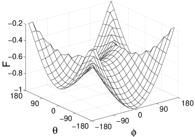
FIG. 3.: Free energy $F$ as a function of $\theta$ and $\phi$ at zero temperature for the toy model 53, with $\beta_{a}=\pi/3$ and $\beta_{b}=\pi/8$. $F$ is plotted in unit of $N_{\rm ch}\Delta_{0}$.

B Chaotic normal layer

Let us now turn to a more realistic model where reflection processes occurring inside the ferromagnetic and normal-metal layers and at their interfaces are fully taken into account, and where scattering from impurities causes the transverse modes to be mixed. In particular, we want to study the effect of spin filtering: the fact that majority and minority electrons have different transmission probabilities for transmission through a ferromagnet layer. (Spin filtering is the dominant source of nonequilibrium current-induced torque for FNF trilayers with normal-metal contacts.) The Josephson current is expected to decrease with increasing reflection inside the FNF trilayer, and with an increasing amount of spin filtering. (Since the Josephson current is carried by Cooper pairs, both the minority and the majority electrons must be transmitted in order to get a current; see Ref. [31] for a discussion of this effect in the context of an FNF trilayer with one superconducting contact.)

Here we assume that the scattering matrix of the normal layer is drawn from the circular orthogonal ensemble from random matrix theory, i.e., in particle/hole grading we set

$${\cal S}_{N}=\mbox{diag}\,(S_{0}\otimes\openone_{2},S_{0}^{*}\otimes\openone_{2}),$$ (57)

where $\openone_{2}$ is the $2\times 2$ identity matrix in spin space and $S_{0}$ is a $2N_{\rm ch}\times 2N_{\rm ch}$ unitary symmetric matrix chosen with uniform probability from the manifold of $2N_{\rm ch}\times 2N_{\rm ch}$ unitary symmetric matrices. The ensemble of scattering matrices corresponds to an ensemble of FNF trilayers with the same $F_{a}$ and $F_{b}$, but different disorder configurations in $N$. The circular ensemble is appropriate for a trilayer where the normal part would be, for example, a dirty metal grain or an amorphous material.[25] When the transmission probabilities of the ferromagnetic layers are small, the circular ensemble can be used for an arbitrary diffusive spacer layer.[25] Our choice of a symmetric scattering matrix implies that the amount of magnetic field leaking into the normal layer from the ferromagnets $F_{a}$ and $F_{b}$ must be sufficiently small, so that time-reversal symmetry is preserved inside $N$. (If time-reversal symmetry is fully broken in $N$, both the supercurrent and the Josephson-effect induced torque will vanish to leading order in $N_{\rm ch}$.)

We are interested in the limit of a large number of channels $N_{\rm ch}$. (For metals, $N_{\rm ch}$ is already of the order of $10^{3}$ for contacts with a width of a few nm.) For large $N_{\rm ch}$, sample-to-sample fluctuations of the current and torque are much smaller than the ensemble average, so that the ensemble averaged current $\bar{I}$ or torque $\bar{\tau}^{\rm equ}$ is sufficient to characterize a single sample. In order to calculate the ensemble average, we first rewrite Eq. (50) in a slightly different form,

$${\rm det}[1-{\cal S}_{FS}(\epsilon)S_{N}]=0,$$ (58)

where ${\cal S}_{FS}(\epsilon)$ is the $8N_{\rm ch}\times 8N_{\rm ch}$ matrix describing the combined effect of scattering from both ferromagnetic layers backed by the superconductors, as seen from the normal spacer layer. The matrix ${\cal S}_{FS}$ has spin, particle/hole ($e-h$), channel, and “$a-b$” degrees of freedom, the latter grading referring to whether scattering is from $F_{a}$ or from $F_{b}$. In the $a-b$ grading, ${\cal S}_{FS}(\epsilon)$ reads,

$${\cal S}_{FS}=\left(\begin{array}[]{cc}{\cal S}_{{FS},a}&0\\ 0&{\cal S}_{{FS},b}\end{array}\right),$$ (59)

with

$${\cal S}_{{FS},a}=r^{\prime}_{a}+t_{a}\frac{1}{1-r_{A}(\phi/2)r_{a}}r_{A}(\phi/2)t^{\prime}_{a},$$ (60)

and

$${\cal S}_{{FS},b}=r_{b}+t^{\prime}_{b}\frac{1}{1-r_{A}(-\phi/2)r_{b}}r_{A}(-\phi/2)t_{b}.$$ (61)

With these notations, the ensemble averaged Josephson current reads,

$$\overline{I}=\frac{2e}{\hbar}kT\sum_{n=0}^{\infty}{\rm Tr}\ \frac{\partial{\cal S}^{-1}_{FS}}{\partial\phi}({\cal S}_{FS}-\overline{{\cal G}}),$$ (62)

with

$${\cal G}=\frac{1}{1-{\cal S}_{FS}{\cal S}_{N}}{\cal S}_{FS}.$$ (63)

The average $\overline{\cal G}$ is computed in the appendix using the method of Ref. [29]. The results of that calculation is a self-consistent equation for $\overline{\cal G}$, analogous to the Dyson equation for the average Green function in a standard impurity average,

$$\overline{{\cal G}}=\frac{1}{1-{\cal S}_{FS}\Sigma}{\cal S}_{FS}$$ (65)

where

$$\Sigma={1\over 2{\bf P}(\overline{{\cal G}})}\left(\sqrt{1+4[{\bf P}(\overline{{\cal G}})]^{2}}-1\right)$$ (66)

and ${\bf P}$ is a projection operator. In $e-h$ space, ${\bf P}$ reads

$${\bf P}\left(\begin{array}[]{cc}A_{ee}&A_{eh}\\ A_{he}&A_{hh}\end{array}\right) = {1\over 2N_{\rm ch}}\mbox{tr}_{N_{\rm ch},ab}\left(\begin{array}[]{cc}0&A_{eh}\\ A_{he}&0\end{array}\right)$$ (72)

$$\mbox{}\otimes 1_{ab}\otimes 1_{N_{\rm ch}},$$

where the trace $\mbox{tr}_{N_{\rm ch},ab}\ldots$ is taken in channel and $a-b$ space, but not in spin space or particle/hole space.

Equation (63) reduces to a self-consistent equation for the $4\times 4$ matrix $\Sigma$. This equation remains fairly complicated and, in general, has to be solved numerically, even when ${\cal S}_{FS}$ is diagonal in channel space. In the limit where ${\cal S}_{FS}$ is close to the identity matrix, i.e., when both ferromagnetic layers are poorly transparent and reflect majority and minority electrons with almost the same reflection phase, a further simplification of Eq. (63) is possible. Assuming that ${\cal S}_{FS}$ is diagonal in channel space (i.e., the ferromagnetic layers do not mix channels), expanding ${\cal S}_{FS}=1+\delta{\cal S}_{FS}+O(\delta{\cal S}_{FS})^{2}$, and defining the $4\times 4$ matrix $X=1/(2N_{\rm ch})\mbox{tr}_{N_{\rm ch},ab}\delta{\cal S}_{FS}$, Eq. (63) reduces to

$$X_{he}+\Sigma_{he}X_{ee}+X_{hh}\Sigma_{he}+\Sigma_{he}X_{eh}\Sigma_{he} = 0,$$ (73)

$$X_{eh}+\Sigma_{eh}X_{hh}+X_{ee}\Sigma_{eh}+\Sigma_{eh}X_{he}\Sigma_{eh} = 0,$$ (74)

while $\Sigma_{ee}=\Sigma_{hh}=0$ since $\Sigma={\bf P}(\Sigma)$. Equation (74) shows that for opaque FN interfaces and for diffusive scattering from the normal spacer layer, there is only a restricted number of parameters (i.e., the free parameters of $X_{eh}$; $X_{he}$ is related to $X_{eh}$ by particle-hole symmetry) that determines the supercurrent and the equilibrium torque.

We could only obtain a solution in closed form in the case where transmission and reflection amplitudes of the ferromagnetic layers were real, i.e., still allowing different transmission and reflection probabilities for majority and minority electrons (spin filtering), but without spin-dependent phase shifts in $F_{a}$ and $F_{b}$. Introducing the mode-averaged transmission probabilities $T_{a\uparrow}$ ($T_{a\downarrow}$) for majority (minority) electrons,

$$T_{a\uparrow}={1\over N_{\rm ch}}\mbox{tr}\,t_{a\uparrow}^{\vphantom{\dagger}}t_{a\uparrow}^{\dagger},\ \ T_{a\downarrow}={1\over N_{\rm ch}}\mbox{tr}\,t_{a\downarrow}^{\vphantom{\dagger}}t_{a\downarrow}^{\dagger},$$

the spin-averaged transmission probability $G_{a}=(T_{a\uparrow}+T_{a\downarrow})/2$, and the geometric mean $\gamma_{a}=(T_{a\uparrow}T_{a\downarrow})^{1/2}$, with similar definitions for $T_{b\uparrow}$, $T_{b\downarrow}$, $G_{b}$, and $\gamma_{b}$, we find

$$\overline{I} = \frac{2e}{\hbar}kTN_{\rm ch}\Delta_{0}\sum_{n=0}^{\infty}\frac{\sin\phi}{\sqrt{\Delta_{0}^{2}+\omega_{n}^{2}}}$$ (76)

$$\mbox{}\times\frac{\gamma_{a}\gamma_{b}}{\sqrt{\gamma_{a}^{2}+\gamma_{b}^{2}+2\gamma_{a}\gamma_{b}\cos\phi+(\omega_{n}/\Delta_{0})^{2}(G_{a}+G_{b})^{2}}}.$$

Equation (76) is the generalization of Equation (24) of Ref. [27] to the case of contacts with spin-dependent transmission, in the short junction limit (Thouless energy much larger than superconducting gap $\Delta_{0}$). In the limit of zero temperature, it reduces to a complete elliptic integral of the first kind. We note that the Josephson current (76) does not depend on the angle $\theta$, so that there is no equilibrium torque in this case. Since the assumption underlying Eq. (76) was that the electrons do not pick up phase shifts in the ferromagnetic regions, we conclude that spin-filtering alone (i.e., the fact that majority and minority electrons have different transmission probabilities) is not enough to create a (Josephson current induced) equilibrium magnetic exchange interaction. We numerically checked that this conclusion still holds when ${\cal S}_{FS}$ is not close to unity.

C Numerical results

For a numerical solution of Eq. 63 that accounts for the fact that majority and minority electrons experience different phase shifts while scattering from the ferromagnetic layers, it would be desirable to have detailed knowledge of the scattering matrices $S_{a}$ and $S_{b}$ of the ferromagnetic layers. These scattering matrices can, in principle, be calculated from ab-initio calculations, see, e.g., Ref. [26]. However, complete data for all amplitudes (phase shifts and probabilities) are not available in the literature. Therefore, we choose an ansatz for $S_{a}$ and $S_{b}$ that is close in spirit to the toy model of Sec. IV A. The use of a simple ansatz can be partly justified by Eq. (74), which shows that it is only a finite number of parameters that determines the supercurrent and exchange interaction, not the entire matrix $S_{a}$ or $S_{b}$. For our ansatz, we assume that these scattering matrices are diagonal in channel space and we neglect any channel dependence. We further assume that most of the reflection processes take place at the FN interface. Without loss of generality, we may set the phase picked up by minority electrons while traversing the ferromagnetic layers equal to zero. Then the difference between minority and majority electrons is fully described by the phases $\beta_{a(b)}$ picked up by majority electrons. This leads us to the ansatz (in left-mover/right-mover space)

$$S_{b\uparrow,ee} = \left(\begin{array}[]{cc}\sqrt{1-T_{b\uparrow}}&i\sqrt{T_{b\uparrow}}e^{i\beta_{b}}\\ i\sqrt{T_{b\uparrow}}e^{i\beta_{b}}&\sqrt{1-T_{b\uparrow}}e^{2i\beta_{b}}\end{array}\right)\otimes\openone_{N_{\rm ch}},$$ (79)

$$S_{b\downarrow,ee} = \left(\begin{array}[]{cc}\sqrt{1-T_{b\downarrow}}&i\sqrt{T_{b\downarrow}}\\ i\sqrt{T_{b\downarrow}}&\sqrt{1-T_{b\downarrow}}\end{array}\right)\otimes\openone_{N_{\rm ch}},$$ (82)

and similar equations for $S_{a\uparrow,ee}$ and $S_{a\downarrow,ee}$, while the scattering matrices $S_{b\uparrow,hh}$, $S_{b\downarrow,hh}$, $S_{a\uparrow,hh}$, $S_{a\downarrow,hh}$ are given by the complex conjugates, cf. Eq. (40).

With this model for the scattering matrices $S_{a}$ and $S_{b}$, a typical plot of the supercurrent at $\phi=\pi/2$ as a function of $\theta$ is shown in Fig. 4. We have taken the values of the parameters $T_{a\uparrow}$, $T_{a\downarrow}$, $T_{b\uparrow}$, and $T_{b\downarrow}$ from realistic estimates for a Co-Cu-Co trilayer,[26, 32] while we fixed the phases $\beta_{a}$ and $\beta_{b}$ arbitrarily. Although the choice of parameters is specific, the observation that the Josephson effect induces a magnetic exchange interaction between the ferromagnetic layers was found to hold for any generic choice of scattering parameters. [The only exception being the case discussed around Eq. (76), for which all scattering phase shifts are either $0$ or $\pi$.] Further, we found that when the phase difference between minority and majority electrons becomes of order unity, the variation of the supercurrent $I$ with $\theta$ is of the order of the critical current, so that, up to a numerical factor, the magnitudes of maximum equilibrium torque and critical current are related as $\tau^{\rm equ}\sim\hbar I_{\rm crit}/2e$.

FIG. 4.: Supercurrent $I$ at phase difference $\phi=\pi/2$ between the superconducting orderparameters, as a function of the angle $\theta$ between the moments of $F_{a}$ and $F_{b}$. The currents is measured in units of $2eN_{\rm ch}\Delta_{0}/\hbar$. We set $T_{a\uparrow}=0.68$, $T_{a\downarrow}=0.29$, $T_{b\uparrow}=0.68$, $T_{b\downarrow}=0.29$, following ab-initio studies of Ref. [26] for a Co-Cu-Co trilayer. The phases $\beta_{a}$ and $\beta_{b}$ were arbitrary set at $\beta_{a}=35\pi/180$ and $\beta_{b}=115\pi/180$. $kT=0.1\Delta_{0}$.

We now turn to a slightly different model for the normal layer which we study by doing the disorder average numerically using Eq. (51). In this model, [33] which was also used in Refs. [8] and [12], ${\cal S}_{N}$ is given by Eq. (57), where the $2N_{\rm ch}\times 2N_{\rm ch}$ scattering matrix $S_{0}$ is parameterized, in a-b grading, as

$$S_{0}=\left(\begin{array}[]{ll}0&U\\ U^{\rm T}&0\end{array}\right).$$ (83)

Here $U$ is an $N_{\rm ch}\times N_{\rm ch}$ unitary matrix, uniformly distributed in the group of unitary $N_{\rm ch}\times N_{\rm ch}$ matrices. This model, in which the normal metal spacer mixes the transverse modes, but does not cause any backscattering is appropriate, e.g., for rough FN interfaces. As the same model was considered for quantitative estimates in Refs. [8] and [12], this choice for ${\cal S}_{N}$ can be used for a quantitative comparison of the Josephson-effect induced equilbrium torque and the nonequilibrium torques considered in Refs. [8] and [12]. Results are shown in Fig. 5 for the same choice of parameters as in Fig. 4.

For all choices of $S_{a}$ and $S_{b}$ that we considered, we find that the results are well described by the phenomenological relation

$$\frac{\partial\tau_{a}^{\rm equ}}{\partial\phi}=\frac{\hbar}{2e}\frac{\partial I}{\partial\theta}\approx N_{\rm ch}\Delta_{0}\sin\phi(J_{1}\sin\theta+J_{2}\sin 2\theta),$$ (84)

where the constants $J_{1}$ and $J_{2}$, which are analogous to the quadratic and bi-quadratic coupling constants in the standard magnetic exchange interaction, depend on the detailed choices for $S_{a}$ and $S_{b}$. Several properties of this phenomenological relation are worth while mentioning. (i) The torque induced by the Josephson current is proportional to the number of transverse channels $N_{\rm ch}$, and hence to the width of the trilayer $N_{\rm ch}$. (This property holds if the ferromagnets are sufficiently weak or thin, so that the phase difference experienced by majority and minority spins is $\lesssim 1$, see the discussion at the end of Sec. IV A.) This should be contrasted with the regular exchange interaction which does not increase with increasing $N_{\rm ch}$ for a disordered normal-metal spacer.[8] Thus, for wide junctions, the Josephson torque is parameterically larger than the standard magnetic exchange interaction. (ii) The torque $\tau^{\rm equ}$ vanishes at $\theta=0$ and $\theta=\pi$, irrespective of $\phi$, since for these angles only spin currents parallel to the magnetic moments play a role, which are conserved. (iii) Similarly, the Josephson current $I$ vanishes at $\phi=0$ and $\phi=\pi$, irrespective of $\theta$. (iv) The Josephson current depends on the angle $\theta$. In the case shown in Fig. 5, the junction shows $\pi$-junction behavior for $\theta=0$, which disappears when $\theta$ approaches $\pi$. The relative strength of the $\theta$-dependent and $\theta$-independent part of the current varies with the phases $\beta_{a}$ and $\beta_{b}$, and the $\pi$-junction behavior is not necessarily there for all choices of $\beta_{a}$ and $\beta_{b}$.

FIG. 5.: Josephson current $I$ and equilibrium torque $\tau^{\rm equ}$ for the model (83) for the scattering matrix of the normal-metal spacer layer, and with the same choice of $S_{a}$ and $S_{b}$ as in Fig. 4. From up to down, the panels contain: $I(\phi)$ for $\theta=\pi/2$, $I(\theta)$ for $\phi=\pi/2$, $\tau^{\rm equ}_{a}(\phi)$ for $\theta=\pi/2$ and $\tau^{\rm equ}_{a}(\theta)$ for $\phi=\pi/2$. For the choice of parameters used for this figure, the Josephson current and the equilibrium torque can be fitted with the phenomenological relation (84), with $J_{1}=0.007$ and $J_{2}=0.025$. Torques are given in units of $\Delta_{0}N_{\rm ch}$ and currents in units of $2e\Delta_{0}N_{\rm ch}/\hbar$. $kT=0.1\Delta_{0}$.

V Conclusion and discussion

We have shown that for a ferromagnet–normal-metal–ferromagnet (FNF) trilayer coupled to two superconducting contacts, the Josephson effect enhances and controls the magnetic exchange interaction between the magnetic moments of the two ferromagnetic layers.

The Josephson-effect induced torque bears important similarities and differences with the nonequilibrium and equilibrium torques in an FNF trilayer with two normal metal contacts:

• The Josephson-effect induced torque points perpendicular to the plane spanned by the directions $\hat{m}_{a}$ and $\hat{m}_{b}$ of the magnetic moments of the ferromagnetic layers, like the standard equilibrium exchange interaction. On the other hand, the nonequilibrium torque mainly lies inside the plane spanned by $\vec{m}_{a}$ and $\vec{m}_{b}$.

• For the Josephson-effect induced torque (or the standard equilibrium exchange interaction) to exist, transmission through the FNF junction needs to be phase coherent. Moreover, existence of the Josephson-effect induced torque requires that majority and minority electrons experience different phase shifts upon transmission through or reflection from the ferromagnetic layers. The nonequilibrium torque, in contrast, only needs spin filtering (different transmission or reflection probabilities for majority and minority electrons), while coherence is not important.[8, 30]

• Like the nonequilibrium torque, the Josephson-effect induced torque is carried by states close to the Fermi energy. The standard equilibrium torque has contributions from states throughout the conduction band.

• The equilibrium torques $\vec{\tau}^{\rm equ}_{a}$ and $\vec{\tau}^{\rm equ}_{b}$ on the moments of both ferromagnetic layers $F_{a}$ and $F_{b}$, respectivly, are equal in magnitude, but opposite in direction, $\vec{\tau}^{\rm equ}_{a}=-\vec{\tau}^{\rm equ}_{b}$. No such relation holds for the nonequilibrium torque.

• The sign and size of the nonequilibrium torque is controlled by the direction of the current. In contrast, the sign of the Josephson effect induced torque is set by the superconducting phase difference $\phi$ and by the details of the scattering phase shifts from the ferromagnetic layers; it is not related to the direction of the supercurrent in any direct way. However, the order of magnitude of the Josephson effect induced torque is set by the size of the critical supercurrent, $\tau^{\rm equ}\sim\hbar I_{\rm crit}/2e$.

We close with a discussion on the effect of the Josephson induced exchange interaction on the dynamics of the magnetic moments. Typically, one of the two ferromagnetic moments (say the moment $\vec{m}_{b}$ of the layer $F_{b}$) is fixed by anisotropy forces, and the torque is studied through its effect on the moment $\vec{m}_{a}$ of the “free” layer $F_{a}$. The usual method to describe the dynamics $\vec{m}_{a}$ in the presence of the current induced torque is via the phenomenological Landau-Lifshitz-Gilbert equation.[5, 34] The result of such a calculation is a critical value of the torque necessary for switching $\vec{m}_{a}$ with respect to the fixed moment $\vec{m}_{b}$. This program was carried out for the non-equilibrium torque acting on a trilayer connected to two normal electrodes in Refs. [5] and [34]. The effect of the equilibrium torque considered here is simpler, as it admits a formulation in terms of the total energy of the system. Using the phenomenological relation (84), the Josephson induced exchange interaction corresponds to an energy gain $\delta f$ per unit area equal to

$$\delta f=\frac{\Delta_{0}}{\lambda_{F}^{2}}\cos\phi\left[J_{1}\hat{m}_{a}\cdot\hat{m}_{b}+J_{2}(\hat{m}_{a}\cdot\hat{m}_{b})^{2}\right].$$ (85)

The criteria for switching the orientation of $\vec{m}_{a}$ is that the magnitude of this interaction energy exceeds that of the work done against anisotropy forces acting on each layer (arising from shape, crystalline structure, etc.). For a $2$ nm thick Cobalt layer, those are of the order of $10^{-3}$ Jm^-2 and can be decreased by up to two orders of magnitude for if Cobalt is replaced by Permalloy [35] Ni₈₁Fe₁₉. On the other hand, for $\Delta_{0}\approx 10K$ (as is the case for Niobium), $\lambda_{F}\approx 1\AA$ and $J_{1}\approx 0.01$ (the value found in our toy model simulations with slightly optimized values for the phase shift differences $\beta_{a}$ and $\beta_{b}$), the Josephson induced interaction is of the order of $10^{-4}$ Jm^-2. Hence, we estimate that control of the relative orientation of $\vec{m}_{a}$ and $\vec{m}_{b}$ should be experimentally accessible provided the local anisotropy forces are kept at a minimum.

When the anisotropy forces are so small that switching of the magnetic moments becomes a possibility, the ac Josephson effect should provide a clear signature of the switching of the ferromagnetic moments through the sensitivity of the supercurrent to the angle $\theta$ between $\vec{m}_{a}$ and $\vec{m}_{b}$. A possible scenario is sketched in Fig. 6: the equilibrium current observed in the Josephson effect should exhibit periodic shifts when the switchings occur. In order to evaluate the fastest time scale at which the switching of the moments can occur, we return to the Landau-Lifshitz-Gilbert equation for the dynamics of the magnetic moments. As before, we suppose that $\vec{m}_{b}$ is kept fixed by a strong local anisotropy field, while the anisotropy field acting on $\vec{m}_{a}$ is negligible. Neglecting the bi-quadratic coupling $J_{2}$, the dynamics of $\vec{m}_{a}$ can then be described by,[5, 34]

$$\frac{\partial\hat{m}_{a}}{\partial t}=\hat{m}_{a}\times\left[\gamma H_{J}(\hat{m}_{a}\cdot\hat{m}_{b})\hat{m}_{b}-\alpha\frac{\partial\hat{m}_{a}}{\partial t}\right].$$ (86)

Here $\gamma=g\mu_{B}/\hbar$ is the gyromagnetic ratio, $\alpha$ the Gilbert damping coefficient and $H_{J}$ is the effective exchange field representing the Josephson-effect induced torque,

$$H_{J}=\frac{J_{1}}{d_{a}|m_{a}|}\cos\phi(t),$$ (87)

where $d_{a}$ is the thickness of the layer $F_{a}$. Neglecting the time dependance of the superconducting phase difference $\phi$, this equation is easily solved,

$$\tan\theta=e^{-\Gamma t}\tan\theta_{0},$$ (88)

with $\Gamma=\gamma H_{J}\alpha/(1+\alpha^{2})$. The switching rate $\Gamma$ is maximum for $\alpha=1$ where, using the numerical values considered above and $|m_{a}|=1.6\ 10^{6}{\rm A/m}$ (for cobalt), we find $\Gamma\approx 10$ GHz. On the other hand, typical voltages used in ac Josephson experiments are of the order of a few $\mu$V, which corresponds to frequencies of the order of a GHz. Therefore, for these frequencies, it should be possible, in principle, to observe the periodic switching of the magnetization orientation as suggested in Fig. 6.

FIG. 6.: Sketch of the current as a function of time when a small voltage $V$ is applied across the junctions. When the Josephson effect induced interaction exceeds the local anisotropy field, the relative configurations of the two moments switches.

Derivation of Eq. (63)

In this appendix, we calculate the ensemble average $\overline{\cal G}$ where ${\cal G}$ is defined in Eq. (63). The ensemble average amounts to the calculation of an average over the circular orthogonal ensemble from random matrix theory (the manifold of unitary symmetric matrices),

$$\overline{{\cal G}}=\int dS_{0}\ {\cal S}_{FS}\frac{1}{1-{\cal S}_{N}{\cal S}_{FS}},$$ (89)

where, in particle/hole ($e-h$) grading, ${\cal S}_{N}=\mbox{diag}\,(S_{0}\otimes\openone_{2},S_{0}^{*}\otimes\openone_{2})$, $\openone_{2}$ being the $2\times 2$ identity matrix in spin space and $S_{0}$ being an $2N_{\rm ch}\times 2N_{\rm ch}$ symmetric unitary matrix, and $dS_{0}$ is the invariant measure for integration over the circular orthogonal ensemble. To perform the average over $S_{0}$, we use the diagrammatic technique of Ref. [29] and calculate $\overline{{\cal G}}$ to leading order in $1/N_{\rm ch}$. First, ${\cal G}$ is expanded in powers of ${\cal S}_{FS}$,

$${\cal G}={\cal S}_{FS}+{\cal S}_{FS}{\cal S}_{N}{\cal S}_{FS}+{\cal S}_{FS}{\cal S}_{N}{\cal S}_{FS}{\cal S}_{N}{\cal S}_{FS}+\ldots$$ (90)

and the corresponding terms are associated with diagrams: a full line corresponds to a factor ${\cal S}_{FS}$ and a dotted line to factor ${\cal S}_{N}$, see Fig. 7a. At each dot one sums over a latin index ranging from $1$ to $2N_{\rm ch}$, representing the channel space, and a greek index ranging from $1$ to $4$, representing the combination of $e-h$ and spin space. According to the diagrammatic rules of Ref. [29], the average is then done by connecting all dots by thin lines, summing over all possible ways of pairing up the dots. To leading order in $1/N_{\rm ch}$, only planar diagrams contribute, i.e., the diagrams where the thin lines do not cross. When two dots are connected, the corresponding latin indices are identified and summed over, and the constraint is imposed that two greek indices involved have to be different in $e-h$ space (i.e., if one index corresponds to $e$, the other one has to correspond to $h$). The rationale for this constraint is that only contractions that involve $S_{0}$ and its complex conjugate are allowed in the average. Finally, a weight factor is associated with each diagram: each cycle formed by an alternation of dotted lines and thin solid lines in the diagram contributes a factor $W_{i}$, where $i$ is equal to half the number of dotted lines contained in the cycle. The $W_{i}$ are tabulated in Ref. [29]; for the purpose of this integral, we only need their generating function[36]

$$\sum_{i=1}^{\infty}W_{i}z^{i-1}=\left(\sqrt{(2N_{\rm ch})^{2}+4z}-(2N_{\rm ch})\right)/2z.$$ (91)

The weight factors $W_{i}$ with $i>1$ correspond to contributions to the average that go beyond a Gaussian evaluation using Wick’s theorem.

(a)

(b)

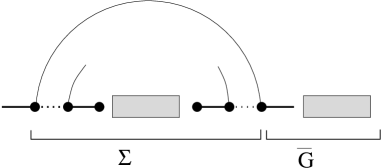
(c)

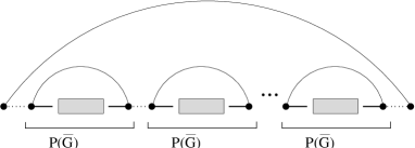
(d)

FIG. 7.: (a) Diagrammatic representation of Eq. (90). (b) The first two diagrams contribution to $\overline{\cal G}$. (c) General structure of diagrams contributing to $\overline{\cal G}$. (d) General structure of diagrams contributing to $\Sigma$.

The first non vanishing diagrams are shown in Fig. 7b. They correspond to

$$\overline{G}={\cal S}_{FS}+2N_{\rm ch}W_{1}\ {\cal S}_{FS}\ {\bf P}({\cal S}_{FS})\ {\cal S}_{FS}+\ldots.$$ (92)

The projector operator ${\bf P}$ was introduced in Eq. (72). It implements the constraint that only greek indices representing $e$ and $h$ degrees of freedom can be contracted.

Now, we are ready to obtain the self-consistent equation (63) for $\overline{G}$. Except from the zeroth order (first term in Eq. (92), all the diagrams involved in $\overline{G}$ have the structure shown in Fig. 7c, where the boxes stand for all possible allowed contractions. The important point here is that there is no thin line connecting the two different boxes since we are only considering planar diagrams. The sum over all the different contractions represented by the right box gives all the possible diagrams and therefore equals $\overline{{\cal G}}$ itself. Denoting the left part of Fig. 7c by $\Sigma$, we have

$$\overline{{\cal G}}={\cal S}_{FS}+{\cal S}_{FS}\Sigma\overline{{\cal G}},$$ (93)

which is Eq. (65). The diagrams contributing to $\Sigma$ have the structure shown in Fig. 7d. They contain $2n-1$ building blocks, $n=1,2,\ldots$, with weight factor $W_{n}$. (Only odd numbers appear, because of the constraint that only indices belonging to $S_{0}$ and its complex conjugate can be contracted.) Each building block can be identified with ${\bf P}({\cal\overline{G}})$. Hence,

$$\Sigma=\sum_{n=1}^{\infty}W_{n}{\rm Tr}\ \left[2N_{\rm ch}{\bf P}(\overline{{\cal G}})\right]^{2n-1},$$ (94)

which leads to Eq. (66) if we use the generating function (91) for the weight factors $W_{n}$.

REFERENCES

- [1] P. Bruno, Phys. Rev. B 52, 411 (1995).
- [2] M.D. Stiles, Phys. Rev. B 48, 7238 (1993).
- [3] J.C. Slonczewski, J. Magn. Magn. Mater. 150, 13 (1995).
- [4] S.O. Demokritov, J. Phys. D: Apl. Phys. 31, 925 (1998).
- [5] J. Slonczewski, J. Magn. Magn. Mater. 159, L1 (1996).
- [6] E.B. Myers, D.C. Ralph, J.A. Katine, R.N. Louie, and R.A. Buhrman, Science 285, 867 (1999).
- [7] J.A. Katine, F.J. Albert, R.A. Buhrman, E.B. Myers, and D.C. Ralph, Phys. Rev. Lett. 84, 3129 (2000).
- [8] X. Waintal, E.B. Myers, P.W. Brouwer, and D.C. Ralph, Phys. Rev. B 62, 12317 (2000)
- [9] For a review, see the collection of articles in IBM J. Res. Dev. 42 (1998) or F.J. Himpsel, J.E. Ortega, G.J. Mankey and R.F. Willis, Adv. in Phys. 47, 511 (1998).
- [10] J.C. Slonczewski, Phys. Rev. B 39, 6995 (1989).
- [11] M. Buttiker, Y. Imry and R. Landauer, Phys. Lett. 96A, 365 (1983).
- [12] X. Waintal and P.W. Brouwer, Phys. Rev. B 63, 220407R (2001).
- [13] X. Waintal and P.W. Brouwer, to appear in the proceedings of the XXXVIth Rencontres de Moriond edited by T. Martin and G. Montambaux. cond-mat/0107265.
- [14] V.V. Ryazanov V.A. Oboznov, A.Yu. Rusanov A.V. Veretennikov, A.A. Golubov and J. Aarts, Phys. Rev. Lett. 86, 2427 (2001).
- [15] I.O. Kulik, Sov. Phys. JETP 22, 841 (1966).
- [16] H. Shiba and T. Soda, Prog. Theor. Phys. 41, 25 (1969).
- [17] A.A. Clerk and V. Ambegaokar, Phys. Rev. B 57, 9109 (2000).
- [18] Y. Tanaka and S. Kashiwaya, Physica C 274, 357 (1997).
- [19] T. Kontos, M. Aprili, J. Lesueur and X. Grison, Phys. Rev. Lett. 86, 304 (2001)
- [20] F.S. Bergeret, A.F. Volkov and K.B. Efetov, Phys. Rev. Lett. 86, 3140 (2001).
- [21] E.A. Koshina and V.N. Krivoruchko, Phys. Rev. B 63, 224515 (2001).
- [22] P.G. de Gennes, Superconductivity of metals and alloys, (Benjamin, New York 1966).
- [23] K.K. Likharev, Rev. Mod. Phys. 51, 101 (1979).
- [24] C.W.J. Beenakker and H. van Houten, in Nanostructures and Mesoscopic Systems, ed W.P. Kirk. Academic, New York 1992.
- [25] C.W.J. Beenakker, Rev. Mod. Phys. 69, 731 (1997).
- [26] M.D. Stiles, J. Appl. Phys. 79, 5805 (1996); Phys. Rev. B. 54, 14679 (1996).
- [27] P.W. Brouwer and C.W.J. Beenakker Chaos, Solitons and Fractals 8, 1249 (1997). Note that an overall factor is missing in Eq.(8). See cond-mat/9611162 for the correct equation.
- [28] C.W.J. Beenakker, in Transport Phenomena in Mesoscopic Systems. Ed. H. Fukuyama and T. Ando. (Springer Berlin 1992).
- [29] P.W. Brouwer and C.W.J. Beenakker, J. Math. Phys. 37, 4904 (1996).
- [30] A. Brataas, Y.V. Nazarov, and G.E.W. Bauer, Phys. Rev. Lett. 84, 2481 (2000).
- [31] F. Taddei, S. Sanvito, J.H. Jefferson and C.J. Lambert, Phys. Rev. Lett. 82, 4938 (1999); V.I. Fal’ko, C.J. Lambert and A.F. Volkov, Phys. Rev. B 60 15394 (1999).
- [32] A Co-Cu-Co trilayer might not be the best choice of materials for this effect because the Curie temperature of Co is rather large. However, to our knowledge, no ab-initio data for weakly ferromagnetic trilayers are available in the literature.
- [33] A.D. Stone, P.A. Mello, K.A. Muttalib, and J.-L. Pichard in Mesoscopic Phenomena in Solids, edited by B. L. Altshuler, P. A. Lee, and R. A. Webb (North Holland, Amsterdam, 1991).
- [34] Ya.B. Bazaliy, B.A. Jones and Shou-Cheng Zhang, Phys. Rev B 57 R3213 (1998).
- [35] D. Jiles Introduction to magnetism and magnetic materials, (Chapman and Hall 1991).
- [36] The generating function can be easily obtained by calculating the average of .