Ensemble properties of securities traded in the NASDAQ market

Abstract

We study the price dynamics of stocks traded in the NASDAQ market by considering the statistical properties of an ensemble of stocks traded simultaneously. For each trading day of our database, we study the ensemble return distribution by extracting its first two central moments. According to previous results obtained for the NYSE market, we find that the second moment is a long-range correlated variable. We compare time-averaged and ensemble-averaged price returns and we show that the two averaging procedures lead to different statistical results.

and

1 Introduction

In recent years physicists started to interact with economists to concur to the modeling of financial markets as model complex systems [1, 2]. A reliable model of a financial market should be able to reproduce and to explain the stylized facts observed in the real markets. These stylized facts mainly refer to the statistical properties of asset returns and volatility and to the degree and nature of cross-correlation between different assets traded synchronously or quasi synchronously and belonging to given portfolios. Recently, we have proposed to look at a different aspect of an ensemble of stock by considering the statistical properties (shape, moments, etc.) of the ensemble return distribution of stocks simultaneously traded in a market [3, 4, 5, 6]. Our studies have shown that some of the statistical properties of the ensemble return distribution of stocks traded in the NYSE market are not described by simple market models as the single-index model [7, 8]. A similar conclusion has been reached in Ref. [9]. In this paper we study the statistical properties of the ensemble return distribution of the NASDAQ market in the 12-year period 1987-1998. The main motivation for this study is to compare our previous findings obtained for the NYSE with the empirical results observed in a different market. The NASDAQ market is very different from the NYSE. Stocks traded in the NASDAQ are usually more volatile (mean volatility is $4.6\%$ per year) than those traded in the NYSE (mean volatility is $2.4\%$ per year). In 1987 the NASDAQ was a relatively small market but its total capitalization and the number of traded companies increased very fast and in 1994 NASDAQ surpassed the NYSE in annual share volume.

2 Ensemble return distribution properties for the NASDAQ

The investigated market is the NASDAQ during the 12-year period from January 1987 to December 1998 which corresponds to 3032 trading days. We consider the ensemble of all stocks traded in the NASDAQ. The number of stocks traded in the NASDAQ is increasing in the investigated period and it ranges from $864$ at the beginning of 1987 to $4280$ at the end of 1998. The total number of data records exceeds $6$ millions. The variable investigated in our analysis is the daily price return, which is defined as

$$R_{i}(t)\equiv\frac{Y_{i}(t+1)-Y_{i}(t)}{Y_{i}(t)},$$ (1)

where $Y_{i}(t)$ is the closure price of $i-$th stock at day $t$ ($t=1,2,..$). For each trading day $t$, we consider $n_{t}$ returns, where $n_{t}$ is the total number of stocks traded in the NASDAQ at the selected day $t$. In our study we use a “market time”. With this choice, we consider only the trading days and we remove the weekends and the holidays from the calendar time. A database of more than 6 millions records unavoidably contains some errors. A direct control of a so large database is not realistic. For this reason, to avoid spurious results we filter the data by not considering daily price returns which are in absolute values greater than $50\%$. We extract the $n_{t}$ returns of the $n_{t}$ stocks for each trading day $t$. The probability density function (pdf) of these returns $P_{t}(R)$ provides information about the kind of activity occurring in the market at the selected trading day $t$. Figure 1 shows the contour plot of the logarithm of the pdf as a function of the return and of the trading day. In Fig. 1 there are long time periods, see for example the three-year period 1993-1995, in which the central part of the distribution maintains its shape and the equiprobability contour lines are approximately parallel one to each other. On the other hand there are time periods in which the shape of the distribution changes drastically. In general these periods corresponds to financial turmoil in the market [4].

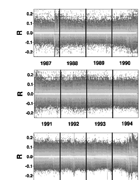
Figure 1: Contour plot of the logarithm of the ensemble return distribution for the 12-year investigated period from January 1987 to December 1998. The contour plot is obtained for equidistant intervals of the logarithmic probability density. The brightest area of the contour plot corresponds to the most probable value.

In order to characterize more quantitatively the ensemble return distribution at day $t$, we extract the first two central moments at each of the $3032$ trading days. Specifically, we consider the mean and the standard deviation of $R_{i}(t)$ defined as

$$\mu(t)=\frac{1}{n_{t}}\sum_{i=1}^{n_{t}}R_{i}(t),$$ (2)

$$\sigma(t)=\sqrt{\frac{1}{n_{t}}\left(\sum_{i=1}^{n_{t}}(R_{i}(t)-\mu(t))^{2}\right)}.$$ (3)

The mean of price returns $\mu(t)$ quantifies the general trend of the market at day $t$. The standard deviation $\sigma(t)$ gives a measure of the width of the ensemble return distribution. We call this quantity variety [3, 5] of the ensemble because it gives a measure of the variety of behavior observed in a financial market at a given day. A large value of $\sigma(t)$ indicates that different companies are characterized by rather different returns at day $t$. The mean and the standard deviation of price returns are not constant and fluctuate in time. The probability density function of the mean $\mu(t)$ is leptokurtic because of the correlation between stocks. In agreement with previous results on the NYSE market [3, 5], we find that the mean $\mu(t)$ is a random variable with very short time memory, whereas the autocorrelation function of $\sigma(t)$ is a slow decaying function and lacks a typical time scale.

Figure 2: Time evolution of the variety $\sigma(t)$ for the NASDAQ market (top) and for a surrogate market generated according to the non Gaussian single index model of Eq. (6) (bottom).

Figure 2 shows the time series of the variety $\sigma(t)$ for the NASDAQ. The time series of the variety is non stationary and shows several bursts of activity and relatively long time periods in which the variety has a slow dynamics. The effects of these observations are reflected in the properties of the autocorrelation function. We observe that the autocorrelation function of the variety is greater than $0.25$ after $100$ trading days.

Figure 3: In the left panel we show the probability density function of the mean $\mu(t)$ of the ensemble return distribution (white diamond) and of the mean of the daily return $\mu_{i}$ of all the stocks traded in the NASDAQ (black square). (right) The right panel is the probability density function of the variety $\sigma(t)$ , i.e. the variance of the ensemble return distribution (white diamond) and of the volatility $\sigma_{i}$, i.e. the variance of the daily return, of the all the stocks traded in the NASDAQ (black square).

It has been shown by us [5] that information about the relative strength of cross-correlation between different stocks and the autocorrelation of price returns can be obtained by comparing the statistical properties of time-averaged and ensemble-averaged quantities. To this end for each stock traded in the NASDAQ we extract the first two central moments of the time series $R_{i}(t)$ defined as

$$\mu_{i}=\frac{1}{t^{b}_{i}-t^{a}_{i}}\sum_{t=t^{a}_{i}}^{t^{b}_{i}}R_{i}(t),$$ (4)

$$\sigma_{i}=\sqrt{\frac{1}{t^{b}_{i}-t^{a}_{i}}\left(\sum_{t=t^{a}_{i}}^{t^{b}_{i}}(R_{i}(t)-\mu_{i})^{2}\right)},$$ (5)

where $t^{a}_{i}$ indicates the first trading day of our database or the day at which the asset $i$ entered the market and $t^{b}_{i}$ indicates the last trading day of our database or the day at which the asset $i$ quit the NASDAQ market. The quantity $\mu_{i}$ gives a measure of the overall performance of stock $i$ in the period. The standard deviation $\sigma_{i}$ is called historical volatility in the financial literature and quantifies the risk associated with the $i$-th stock. This quantity is of primary importance in risk management and in option pricing. The left panel of Figure 3 shows the pdf of the time-averaged mean $\mu_{i}$ and the pdf of the ensemble-averaged mean $\mu(t)$. The pdf of $\mu_{i}$ is non-Gaussian and it is much more peaked than the pdf of $\mu(t)$. Hence the statistical behavior observed by investigating a large ensemble in a market day is not representative of the statistical behavior observed by investigating the time evolution of single stocks. This comparison can be performed also for the second moment of the distributions. In the right panel of Figure 3 we compare the pdf of the volatility $\sigma_{i}$ and the pdf of the variety $\sigma(t)$. Also in this case, the statistical properties of $\sigma_{i}$ and $\sigma(t)$ are different. Specifically, the pdf of $\sigma(t)$ is more peaked than the pdf of $\sigma_{i}$. We showed [5] that the width of the pdf of $\mu(t)$ is related to the mean synchronous cross-covariance between pairs of stock returns, whereas the width of the pdf of $\mu_{i}$ is related to the mean autocorrelation of stock return time series. The left panel of Figure 3 confirms that also for the NASDAQ market the synchronous cross-correlations between the stocks are on average stronger than the single stock correlation present in the whole portfolio at two different trading day. In order to test how robust are these conclusion on the time horizon used to define returns, we perform the same analysis by considering weekly (5 trading days) returns and we find the same discrepancy between the pdfs of time averaged and ensemble averaged quantities. In the following we compare our results with the results obtained by modeling the price dynamics with a single index model [7, 8]. The single-index model assumes that the returns of all assets are controlled by one factor. For any asset $i$, we have

$$R_{i}(t)=\alpha_{i}+\beta_{i}R_{M}(t)+\epsilon_{i}(t),$$ (6)

where $R_{i}(t)$ and $R_{M}(t)$ are the return of the asset $i$ and of the market factor at day $t$, respectively, $\alpha_{i}$ and $\beta_{i}$ are two real parameters and $\epsilon_{i}(t)$ is a zero mean noise term characterized by a variance equal to $\sigma^{2}_{\epsilon_{i}}$. Our choice for the market factor is the NASDAQ 100 index and we assume that $\epsilon_{i}=\sigma_{\epsilon_{i}}w$, where $w$ is a random variable distributed according to a Student’s t density function with exponent such that $P(w)\sim w^{-4}$. The use of a non Gaussian noise term has been recently proposed in Ref. [9]. We estimate the model parameters for each asset and we generate an artificial market according to Eq. (6). A similar analysis has been performed in Ref. [5] for the NYSE market. We find that the single index model explains well the statistical properties of $\mu_{i}$, $\mu(t)$ and $\sigma_{i}$ but fails in describing the statistical properties of variety $\sigma(t)$. In the bottom panel of Figure 2 we show the variety of a surrogate market generated according to Eq. (6). The time series is very different from the real one showed in the top panel of the same Figure.

3 Conclusion

The present study performs an analysis the dynamics of returns of an ensemble of stocks traded in the NASDAQ. We observe that also in the NASDAQ the variety is a long-range correlated stochastic variable and that time-averaged and ensemble-averaged price returns have different statistical properties. Therefore the empirical results found in the NYSE are not specific of that market but are observed also in the NASDAQ. The statistical properties of the variety could be universal features of financial markets. In previous papers [5, 6] we showed that the statistical properties of the variety cannot be explained by the single-index model. A theoretical challenge is to find a model able to explain these empirical ensemble observations.

References

- [1] R. N. Mantegna and H. E. Stanley, An Introduction to Econophysics: Correlations and Complexity in Finance, (Cambridge Univ. Press, 2000).
- [2] J.-P. Bouchaud and M. Potters, Theory of financial risk, (Cambridge Univ. Press, 2000).
- [3] F. Lillo and R. N. Mantegna, International Journal of Theoretical and Applied Finance, 3, 405 (2000).
- [4] F. Lillo and R. N. Mantegna, Eur. Phys. J. B 15, 603 (2000).
- [5] F. Lillo and R. N. Mantegna, Phys. Rev. E 62, 6126 (2000).
- [6] F. Lillo and R. N. Mantegna, Eur. Phys. J. B 20, 503 (2001).
- [7] E. J. Elton and M. J. Gruber Modern Portfolio Theory and Investment Analysis, (J. Wiley & Sons, New York, 1995).
- [8] J. Y. Campbell, A. W. Lo, A. C. MacKinlay The Econometrics of Financial Markets, Princeton University Press (Princeton, 1997).
- [9] P. Cizeau, M. Potters, J.-P. Bouchaud, Quantitative Finance 1, 217 (2001).