Ferromagnetism in the Hubbard Model

Abstract

We investigate the possibility and stability of bandferromagnetism in the single-band Hubbard model. This model poses a highly non-trivial many-body problem the general solution of which has not been found up to now. Approximations are still unavoidable. Starting from a simple two-pole ansatz for the spectral density our approach is systematically improved by focusing on the influence of quasiparticle damping and the correct weak-and strong coupling behaviour. The compatibility of the different aproximative steps with decisive moment sum rules is analysed and the importance of a spin-dependent band shift mediated by higher correlation functions is worked out. Results are presented in terms of temperature- and band occupation-dependent quasiparticle densities of states and band structures as well as spontaneous magnetisations, susceptibilities and Curie temperatures for varying electron densities and coupling strengths. Comparison is made to numerically essentially exact Quantum Monte Carlo calculations recently done by other authors using dynamical mean field theory for infinite-dimensional lattices. The main conclusion will be that the Hubbard model provides a qualitatively correct description of bandferromagnetism if quasiparticle damping and selfconsistent spin-dependent bandshifts are properly taken into account.

1 Introduction

Ferromagnetism is bound to the existence of permanent magnetic moments. If these belong to itinerant electrons in a partially filled conduction band one speaks of bandferromagnetism Cap87 . Archetypical representatives are the classical 3d ferromagnets Fe, Co, Ni. The microscopic interpretation of bandferromagnetism is one of the most interesting and most complicated many-particle problems in solid state physics. The simple but fairly successful “Stoner criterion”

$$U\varrho_{0}(E_{F})>1$$ (1)

(U: intraatomic Coulomb interaction, $\varrho_{0}$: free Bloch-density of states (B-DOS), $E_{F}$: Fermi energy) defines as a minimum set of ingredients for a theoretical model to describe bandferromagnetism the Pauli-principle, the kinetic energy, the Coulomb interaction (strong and strongly screened), and the lattice structure. This minimum set is realized in the Hubbard-Hamiltonian (2) for correlated electrons on a lattice in a non-degenerate energy band,

$$\hat{H}=\sum\limits_{ij,\sigma}(T_{ij}-\mu\delta_{ij})c^{+}_{i\sigma}c_{j\sigma}+\frac{1}{2}U\sum_{i\sigma}n_{i\sigma}n_{i-\sigma}$$ (2)

($\mu$: chemical potential). The Coulomb interaction is restricted to its intraatomic part only $(n_{i\sigma}=c^{+}_{i\sigma}c_{i\sigma})$, while the kinetic energy contains the hopping integrals $T_{ij}$ being strongly related to the lattice structure. The Pauli principle is guaranteed by the formalism of second quantization. $c^{+}_{i\sigma}(c_{i\sigma})$ is the creation (annihilation) operator for an electron with spin $\uparrow$ or $\downarrow$ at lattice site $\vec{R}_{i}$.

The physics of the Hubbard-model is decisively determined by the Coulomb coupling $U/W$ (W: Bloch-bandwidth), the lattice structure and the band occupation $n=\frac{1}{N}\sum_{\sigma}<n_{\sigma}>$ ($0\leq{n}\leq{2}$; N: number of lattice sites).

In spite of its simple structure the Hamiltonian (2) provokes a rather sophisticated many-body problem, that could be solved in the past only for a few special cases. In general approximations are unavoidable. So it was not fully clarified until recently whether or not ferromagnetism is possible in the Hubbard-model for finite U, finite temperatures T and band occupations away from half filling n=1. Nagaoka showed Nag66 for the special case $U=\infty$ and electron numbers $N_{e}=N\pm 1$ on an sc or bcc lattice and $N_{e}=N+1$ on an fcc lattice, respectively, that the fully spin-polarized particle system represents the ground state. However, the (numerical) proof of finite-temperature ferromagnetism in an extended parameter region was only recently given by Ulmke Ul98 for an infinite dimensional $(d=\infty)$ fcc-type lattice by use of Quantum Monte Carlo (QMC) calculations in connection with Dynamical Mean Field Theory (DMFT) MV89 ; M-H89 . On the other hand, the certainty that ferromagnetism exists in the Hubbard model does not at all mean that the phenomenon itself is understood. What is the physical mechanism enforcing ferromagnetic spin order of itinerant electrons? This question can be answered, if at all, better by analytical approaches to the highly complicated electron correlation problem than by purely numerical evaluations. Starting from some basic features we shall construct in the following chapters three different theories for the Hubbard model to contribute to an answer of the above question. The theories are constructed in such a way that each differs from the preceding one by eliminating an obvious shortcoming. We start from a simple spectral density approach (SDA) which suggests itself by some rigorous strong coupling features. However, it suffers from a complete neglect of quasiparticle damping and a wrong weak-coupling behaviour. By use of a modified alloy analogy (MAA) the advantages of the SDA are retained but quasiparticle damping is included. Comparison of the SDA- and the MAA-results helps us to recognize the influence of quasiparticle damping on magnetic stability. The weak coupling behaviour, however, remains insufficient. From a modified perturbation theory (MPT) which correctly reproduces the weak- as well as the strong-coupling limit, we learn by comparison with SDA and MAA how decisive the correct weak coupling (low energy) description is for a theoretical approach that aims at the strong-coupling phenomenon ferromagnetism.

2 Hubbard model basic features

It is commonly accepted that ferromagnetism is a strong-coupling phenomenon. A theoretical approach should therefore be reliable first of all in the ${U\gg W}$ regime. Practically all information we are interested in can be derived from the retarded single-electron Green’s function Mah90

$$G_{\vec{k}\sigma}(E)={\langle\langle{c_{\vec{k}\sigma};c^{+}_{{\vec{k}\sigma}}}\rangle\rangle}_{E}=-{\rm i}\int\limits_{0}^{\infty}dt\exp({\frac{{\rm i}}{\hbar}Et})\langle{[c_{\vec{k}\sigma}(t),c^{+}_{\vec{k}\sigma}(0)]_{+}}\rangle$$ (3)

$$c_{\vec{k}\sigma}={\frac{1}{\sqrt{N}}\sum_{i}c_{i\sigma}\exp(-{\rm i}{\vec{k}\vec{R}_{i}}})$$ (4)

$[..,..]_{+(-)}$ means the anticommutator (commutator) and $\langle..\rangle$ the grandcanonical average. $\vec{k}$ is a wavevector from the first Brillouin zone. Of equivalent importance is the single-electron spectral density being directly related to the bare line shape of an angle- and spin-resolved (direct or inverse) photoemission experiment:

$$S_{\vec{k}\sigma}(E)=-{\frac{1}{\pi}}ImG_{\vec{k}\sigma}(E+{\rm i}0^{+})$$ (5)

According to the pioneering work of Harris and Lange HL67 we know that in the strong coupling limit $S_{\vec{k}\sigma}(E)$ is built up by two main peaks near $T_{0}$ and $T_{0}+U$ where $T_{0}$ is the centre of gravity of the free Bloch band, and additional satellite peaks at $T_{0}+pU$ $(p=-1,-2,\ldots;p=2,3,\ldots)$ (s. Fig.1). The spectral weights ($\propto$ peak area) of the satellites, however, decrease rapidly with increasing distance from the main peaks. Already the next neighbours $(p=-1,+2)$ acquire only a weight of order $({\frac{W}{U}})^{4}$ being therefore negligible in the strong-coupling regime. So we can assume for ${U\gg W}$ a two-peak structure of the spectral density. The exact shapes of the peaks are not known, but the centres of gravity are,

$$T_{1\sigma}(\vec{k})=T_{0}+(1-\langle n_{-\sigma}\rangle)(\varepsilon(\vec{k})-T_{0})+\langle n_{-\sigma}\rangle B_{\vec{k}-\sigma}+0({\frac{W}{U}})^{4}$$ (6)

$$T_{2\sigma}(\vec{k})=T_{0}+U+\langle n_{-\sigma}\rangle(\varepsilon(\vec{k})-T_{0})+(1-\langle n_{-\sigma}\rangle)B_{\vec{k}-\sigma}+0(\frac{W}{U})^{4}$$ (7)

as well as their spectral weights:

$$\alpha_{1\sigma}(\vec{k})=(1-\langle n_{-\sigma}\rangle)+0(\frac{W}{U})=1-\alpha_{2\sigma}(\vec{k})$$ (8)

Figure 1: Single electron spectral density of the Hubbard model in the strong coupling regime ($U\gg W$) as function of energy.

At least formally the centres of gravity carry a spin-dependence which may give rise to an additional exchange splitting of the two main peaks as the fundamental precondition for ferromagnetism. In the following it is demonstrated that such a spin asymmetry is mainly due to the “band correction” $B_{\vec{k}-\sigma}$:

$$B_{\vec{k}-\sigma}=B_{-\sigma}+F_{\vec{k}-\sigma}$$ (9)

The local term $B_{-\sigma}$ (“band-shift”) can be interpreted as a correlated electron hopping:

$$\langle n_{-\sigma}\rangle(1-\langle n_{-\sigma}\rangle)B_{-\sigma}={\frac{1}{N}}\sum\limits_{i,j}^{i{\neq j}}T_{ij}\langle c_{i-\sigma}^{+}c_{j-\sigma}(2n_{i\sigma}-1)\rangle$$ (10)

For $U\gg W$ and less than half-filled bands double occupancies are very unlikely so that the second term in the bracket dominates. That means that the shift of the $\sigma$-spectrum is correlated with the negative kinetic energy of the $(-\sigma)$-electrons. For further evaluations it will turn out to be decisive that the band-shift $B_{-\sigma}$ can exactly be expressed by the single-electron spectral-density GN88 ; NB89

$$\langle n_{-\sigma}\rangle(1-\langle n_{-\sigma}\rangle)B_{-\sigma}=$$ (12)

$${\frac{1}{N\hbar}}\sum_{\vec{k}}(\varepsilon(\vec{k})-T_{0})\int^{\infty}_{-\infty}\mathrm{d}Ef_{-}(E)({\frac{2}{U}}(E-\varepsilon(\vec{k}))-1))S_{\vec{k}-\sigma}(E-\mu)$$

$f_{-}(E)=(\exp{\beta(E-\mu)}+1)^{-1}$ is the Fermi function. $B_{-\sigma}$ obviously disappears in the zero-bandwidth limit$(\varepsilon(\vec{k})\longrightarrow T_{0}\,\forall\,\vec{k})$.

The k-dependent part of the band correction (9) is built up by density-density, double hopping and spinflip correlation terms

$$\langle n_{-\sigma}\rangle(1-\langle n_{-\sigma}\rangle)F_{\vec{k}-\sigma}=$$ (15)

$${\frac{1}{N}}\sum\limits_{i,j}^{i\neq j}T_{ij}\exp(-{\rm i}\vec{k}(\vec{R}_{i}-\vec{R}_{j}))(\langle n_{i-\sigma}n_{j-\sigma}\rangle-\langle n_{j-\sigma}\rangle^{2}$$

$$+\langle c^{+}_{j-\sigma}c^{+}_{j\sigma}c_{i-\sigma}c_{i\sigma}\rangle+\langle c^{+}_{j\sigma}c_{j-\sigma}c^{+}_{i-\sigma}c_{i\sigma}\rangle)$$

It vanishes in the zero-bandwidth limit and has no direct influence on the centres of gravity $T_{1,2\sigma}$ of the quasiparticle subbands (Hubbard bands) that emerge from the two spectral density peaks (Fig. 1):

$$\hat{T}_{1\sigma}={\frac{1}{N}}\sum_{\vec{k}}T_{1\sigma}(\vec{k})=T_{0}+\langle n_{-\sigma}\rangle B_{-\sigma}$$ (16)

$$\hat{T}_{2\sigma}={\frac{1}{N}}\sum_{\vec{k}}T_{2\sigma}(\vec{k})=T_{0}+U+(1-\langle n_{-\sigma}\rangle)B_{-\sigma}$$ (17)

$F_{\vec{k}-\sigma}$ may, however, lead to a spin-dependent bandwidth correction competing then with the other band narrowing terms in (6) and (7), respectively. The importance of $F_{\vec{k}-\sigma}$ with respect to ferromagnetism shall be discussed in Sect.III. Unfortunately, it cannot be expressed by the spectral density as the band shift $B_{-\sigma}$ by eq. (11). A determination of $F_{\vec{k}-\sigma}$ therefore requires further approximations.

If $B_{\vec{k}-\sigma}$ has indeed such vital implications a theoretical approach should handle this term with special care. That can effectively be controlled by the spectral moments of the spectral density,

$$M^{(n)}_{\vec{k}\sigma}={\frac{1}{\hbar}}\int\limits_{-\infty}^{\infty}\mathrm{d}EE^{n}S_{\vec{k}\sigma}(E)\quad n=0,1,2,3,\ldots$$ (18)

which can be calculated independently of $S_{\vec{k}\sigma}(E)$ via

$$M^{(n)}_{\vec{k}\sigma}=\langle[({\rm i}\hbar\frac{\partial}{\partial t})^{n}c_{\vec{k}\sigma}(t),c^{+}_{\vec{k}\sigma}(t^{\prime})]_{+}\rangle_{t=t^{\prime}}$$ (19)

In practice, however, the moments are useful only for low order n because with increasing n eq.(16) produces higher expectation values which are usually unknown and not expressible by the spectral density, either. The important band correction $B_{\vec{k}-\sigma}(E)$ first appears in $M^{(3)}_{\vec{k}\sigma}$ GN88 ; NB89 .

$$M^{(0)}_{\vec{k}\sigma}=1$$ (20)

$$M^{(1)}_{\vec{k}\sigma}=\hat{\varepsilon}(\vec{k})+U\langle n_{-\sigma}\rangle$$ (21)

$$M^{(2)}_{\vec{k}\sigma}=\hat{\varepsilon}^{2}(\vec{k})+2{\hat{\varepsilon}}(\vec{k})U\langle n_{-\sigma}\rangle+U^{2}\langle n_{-\sigma}\rangle$$ (22)

$$M^{(3)}_{\vec{k}\sigma}=\hat{\varepsilon}^{3}(\vec{k})+3\hat{\varepsilon}^{2}(\vec{k})U\langle n_{-\sigma}\rangle+\hat{\varepsilon}(\vec{k})U^{2}\langle n_{-\sigma}\rangle(2+\langle n_{-\sigma}\rangle)$$ (23)

$$\quad\quad+U^{3}\langle n_{-\sigma}\rangle+U^{2}\langle n_{-\sigma}\rangle(1-\langle n_{-\sigma}\rangle)(B_{\vec{k}-\sigma}+T_{0}-\mu)$$ (24)

($\hat{\varepsilon}(\vec{k})=\varepsilon(\vec{k})-\mu$). A necessary condition for a theoretical approach to be consistent with the strong-coupling results (6),(7),(8) is that the first four moments $M^{(n)}_{\vec{k}\sigma},n=0,1,2,3$ are correctly reproduced. The condition becomes even sufficient when additionally the zero-bandwidth limit Hub63 is fullfilled. One can elegantly check the strong coupling consistency by use of the high-energy expansion of the single-electron Green’s function

$$G_{\vec{k}\sigma}(E)=\int\limits_{-\infty}^{+\infty}dE^{\prime}\frac{S_{\vec{k}\sigma}(E^{\prime})}{E-E^{\prime}}\longrightarrow\hbar\sum\limits_{n=0}^{\infty}\frac{M^{(n)}_{\vec{k}\sigma}}{E^{n+1}}$$ (25)

which can also be used in the Dyson equation,

$$G_{\vec{k}\sigma}(E)=G^{(0)}_{\vec{k}}(E)+G^{(0)}_{\vec{k}}(E){\frac{1}{\hbar}}\Sigma_{\vec{k}\sigma}(E)G_{\vec{k}\sigma}(E),$$ (26)

where

$$G^{(0)}_{\vec{k}}(E)=\hbar(E+\mu-\varepsilon(\vec{k}))^{-1}$$ (27)

is the $U=0$  Green’s function, to yield a respective expansion for the selfenergy:

$$\Sigma_{\vec{k}\sigma}(E)=\sum\limits_{m=0}^{\infty}{\frac{C^{(m)}_{\vec{k}\sigma}}{E^{m}}}$$ (28)

The coefficients $C^{(m)}_{\vec{k}\sigma}=f_{m}(M^{(0)}_{\vec{k}\sigma},\ldots,M^{(m+1)}_{\vec{k}\sigma})$ are simple functions of the moments up to order $m+1$:

$$C^{(0)}_{\vec{k}\sigma}=M^{(1)}_{\vec{k}\sigma}-(\varepsilon(\vec{k})-\mu)$$ (29)

$$C^{(1)}_{\vec{k}\sigma}=M^{(2)}_{\vec{k}\sigma}-(M^{(1)}_{\vec{k}\sigma})^{2}$$ (30)

$$C^{(2)}_{\vec{k}\sigma}=M^{(3)}_{\vec{k}\sigma}-2M^{(2)}_{\vec{k}\sigma}M^{(1)}_{\vec{k}\sigma}+(M^{(1)}_{\vec{k}\sigma})^{3}$$ (31)

$$\ldots$$ (32)

For a given theoretical approach one can easily control whether or not the leading term in the expansions (21)and (24), respectively, match with the rigorously calculated moments. However, even the opposite procedure may be useful, infering approximately the overall energy dependence of the Green’s function and the selfenergy, respectively, from the first few exactly calculated terms. A proposal how this can be done is exemplified in the next Section.

Rigorous statements are of course also possible in the weak coupling regime ($U\ll W$). As mentioned in Sect.I it remains a challenging problem to find out how decisive weak coupling and low-energy properties are for a theoretical approach to correctly describe the strong-coupling phenomenon “ferromagnetism”. In the “diagram-language” the Dyson equation (22) reads

$$\qquad G_{\vec{k}\sigma}(E)\qquad\;=\qquad\quad G^{(0)}_{\vec{k}}(E)\qquad+\quad G^{(0)}_{\vec{k}}(E){\frac{1}{\hbar}}\Sigma_{\vec{k}\sigma}(E)G_{\vec{k}\sigma}(E)$$ (33)

Using standard perturbation theory Mah90 ; NoltingBd7 ; AGD64 one has to sum up for the selfenergy $\Sigma_{\vec{k}\sigma}(E)$ all dressed skeleton diagrams. A “skeleton diagram” is a selfenergy diagram that does not contain any selfenergy insertion in its propagators. If in addition the propagators are “full” Green’s functions $G_{\vec{k}\sigma}(E)$ then the skeleton is “dressed”. That means for the Hubbard model up to second order:

Conventional diagram rules Mah90 ; NoltingBd7 ; AGD64 yield as selfconsistent second order perturbation theory in$\frac{U}{W}$:

$$\Sigma_{\vec{k}\sigma}(E)=U\langle n_{-\sigma}\rangle+U^{2}\Delta_{\vec{k}\sigma}(E)+0(U^{3})$$ (34)

The linear term is the Hartree-Fock (Stoner) part while the more complicated second order contribution is in general non-local, complex, and energy dependent:

$$\Delta_{\vec{k}\sigma}(E)=$$ (37)

$$\frac{1}{\hbar^{3}N^{2}}\sum\limits_{\vec{q}\vec{p}}\int\int\int\mathrm{d}\varepsilon_{1}\mathrm{d}\varepsilon_{2}\mathrm{d}\varepsilon_{3}{\frac{S_{\vec{q}+\vec{k}\sigma}(\varepsilon_{1}-\mu)S_{\vec{p}-\sigma}(\varepsilon_{2}-\mu)S_{\vec{p}-\vec{q}-\sigma}(\varepsilon_{3}-\mu)}{E+\mu-\varepsilon_{1}+\varepsilon_{2}-\varepsilon_{3}+{\rm i}0^{+}}}$$

$$\times\big{(}f_{-}(\varepsilon_{1})f_{-}(-\varepsilon_{2})f_{-}(\varepsilon_{3})+f_{-}(-\varepsilon_{1})f_{-}(\varepsilon_{2})f_{-}(-\varepsilon_{3})\big{)}$$

S is the full spectral density which has to be determined self-consistently. Several alternatives are thinkable which are correct and equivalent up to order $U^{2}$. One of these is to replace the “full” spectral density in (29) by its Hartree-Fock version SC90 ; ZH83

$$S^{(1)}_{\vec{k}\sigma}(E)=S^{(0)}_{\vec{k}\sigma}(E-U\langle n_{-\sigma}\rangle^{(1)})$$ (38)

To avoid an ambiguity we require that the Hartree-Fock particle densities are the same as those in the full calculation:

$$\langle n_{\sigma}\rangle^{(1)}=\langle n_{\sigma}\rangle$$ (39)

that can be regulated by considering the chemical potential $\mu^{(1)}$ in (30) as a proper fit parameter. There are of course other possibilities to avoid the mentioned ambiguity KK96 .

Several very important conclusions can be drawn from (28), e.g. for the low-energy behaviour of the selfenergy Lut61 at $T=0\,(\alpha,\beta,\gamma,\,real)$,

$$\Sigma_{\vec{k}\sigma}(E)=\alpha_{\vec{k}\sigma}+\beta_{\vec{k}\sigma}E+{\rm i}\vec{\gamma}_{\vec{k}\sigma}E^{2}+\ldots$$ (40)

That means that the imaginary part of $\Sigma$ disappears at the Fermi edge ($E=0$) indicating quasiparticles with infinite lifetimes. At low but finite temperatures holds

$$Im\Sigma_{\vec{k}\sigma}(0)\propto T^{2}\quad(T\longrightarrow 0)$$ (41)

(32) and (33) are necessary to guarantee the correct Fermi liquid behaviour.

3 Analytical Approaches

We can now use the basic features of the last section to construct and control three different analytical approaches. The main goal is to work out the essentials for ferromagnetism in the Hubbard model by a critical comparison of these theories.

3.1 Spin-dependent band shift

Having in mind the two-peak structure of the spectral density in the strong-coupling regime (Fig.1) we can construct a simple “spectral density approach” (SDA). If we initially assume that quasiparticle damping, responsible for the finite peak widths, does not play a dominant role for magnetic properties then the following two-pole ansatz appears to be plausible:

$$S_{\vec{k}\sigma}(E)=\hbar\sum\limits_{j=1}^{2}\alpha_{j\sigma}(\vec{k})\delta(E+\mu-E_{j\sigma}(\vec{k}))$$ (42)

The quasiparticle energies $E_{j\sigma}(\vec{k})$ and their spectral weigths $\alpha_{j\sigma}(\vec{k})$ are easily fixed by equating the first four moments. The resulting selfenergy has a remarkable structure GN88 ; NB89 ; HN97 ; Ro69 , in particular the important “band correction” $B_{\vec{k}-\sigma}$ is involved:

$$\Sigma^{SDA}_{\vec{k}\sigma}(E)=U\langle n_{-\sigma}\rangle\frac{E+\mu-T_{0}-B_{\vec{k}-\sigma}}{E+\mu-T_{0}-B_{\vec{k}-\sigma}-U(1-\langle n_{-\sigma}\rangle)}$$ (43)

According to (10) and (12) $B_{\vec{k}-\sigma}$ vanishes in the zero-band-width limit ($W\longrightarrow 0$). $\Sigma^{SDA}_{\vec{k}\sigma}(E)$ is then the exact $W=0$ selfenergy Hub63 ; HN97 . Additionally the SDA fullfills by construction the first four moments so that the strong-coupling behaviour must be correct according to (6)-(8).The first three terms of the high-energy expansion of $\Sigma^{SDA}_{\vec{k}\sigma}(E)$ agree exactly with (25)-(27).

We note in passing that the so-called “Hubbard-I approach” Hub63 leads to a selfenergy being identical to that of the $W=0$ limit. It thus coincides with that of the SDA for $B_{\vec{k}-\sigma}=0$. Comparing the results of SDA and Hubbard-I therefore helps to understand the implications due to $B_{\vec{k}-\sigma}$.

Two severe shortcomings of the SDA are also very obvious. The first is the neglect of quasiparticle damping by the delta-function ansatz (34) which leads to a real selfenergy $\Sigma^{SDA}_{\vec{k}\sigma}(E)$. The second concerns the weak-coupling regime, which is surely violated by the strong-coupling theory SDA. It is not to expect that Fermi liquid behaviour is correctly described by the SDA. These two points shall be attacked and eliminated by the subsequent approaches. But let us first inspect what the SDA tells about bandferromagnetism in the Hubbard model.

For a full SDA-solution we have to determine the “band correction” $B_{\vec{k}-\sigma}$(9). The local part $B_{-\sigma}$ does not need a special treatment because of its direct connection (11) to the spectral density itself. The $\vec{k}$-dependent part $F_{\vec{k}-\sigma}$ appears a bit more complicated. Assuming translational invariance and next neighbour hopping, only, the $\vec{k}$-dependence can be separated HN97 ; Ro69 :

$$\langle n_{-\sigma}\rangle(1-\langle n_{-\sigma}\rangle)F_{\vec{k}-\sigma}=(\varepsilon(\vec{k})-T_{0})\sum\limits_{i=1}^{3}F^{(i)}_{-\sigma}$$ (44)

$$F^{(1)}_{-\sigma}=\langle n_{i-\sigma}n_{j-\sigma}\rangle-\langle n_{-\sigma}\rangle^{2}$$ (45)

$$F^{(2)}_{-\sigma}=\langle c^{+}_{j-\sigma}c^{+}_{j\sigma}c_{i-\sigma}c_{i\sigma}\rangle$$ (46)

$$F^{(3)}_{-\sigma}=\langle c^{+}_{j\sigma}c_{j-\sigma}c^{+}_{i-\sigma}c_{i\sigma}\rangle$$ (47)

i,j are numbering next neighbours. The method used to determine the higher correlations $F^{(i)}_{-\sigma}$ shall be exemplified for $F^{(3)}_{-\sigma}$. First we rewrite $F^{(3)}_{-\sigma}$ as

$$F^{(3)}_{-\sigma}=\sum\limits_{l}\delta_{jl}\langle c^{+}_{l\sigma}c_{j-\sigma}c^{+}_{j+\Delta-\sigma}c_{j+\Delta\sigma}\rangle$$ (48)

where the index $\Delta$ corresponds to the lattice vector which connects two neighbouring sites $\vec{R}_{i}$ and $\vec{R}_{j}$. Because of translational invariance $F^{(3)}_{-\sigma}$ does not depend on the explicit value of $\Delta$. We now introduce a “higher” spectral density $S^{(3)}_{\vec{k}\sigma}(E)$ as the ($\vec{k},E$)-dependent Fourier transform of

$$S^{(3)}_{jl\sigma}(t,t^{\prime})=\frac{1}{2\pi}\langle[(c_{j-\sigma}c^{+}_{j+\Delta-\sigma}c_{j+\Delta\sigma})(t),c^{+}_{l\sigma}(t^{\prime})]_{+}\rangle$$ (49)

The spectral theorem yields:

$$F^{(3)}_{-\sigma}=\frac{1}{\hbar N}\sum\limits_{\vec{k}}\int\limits_{-\infty}^{\infty}\mathrm{d}Ef_{-}(E)S^{(3)}_{\vec{k}\sigma}(E-\mu)$$ (50)

According to the definition (41) the poles of $S^{(3)}_{\vec{k}\sigma}(E)$ must belong to the single-electron excitations of the Hubbard system. From the spectral representation of $S^{(3)}_{\vec{k}\sigma}(E)$ and by comparison with the respective representation of the single-electron spectral density $S_{\vec{k}\sigma}(E)$ again a two pole ansatz appears to be consistent,

$$S_{\vec{k}\sigma}(E)=\hbar\sum\limits_{j=1}^{2}\hat{\alpha}_{j\sigma}(\vec{k})\delta(E+\mu-E_{j\sigma}(\vec{k}))$$ (51)

where the quasiparticle energies $E_{j\sigma}(\vec{k})$ are the same as those in (34) so that the spectral weights $\hat{\alpha}_{j\sigma}$ are the only unknown parameters. They are fixed by the first two spectral moments of $S^{(3)}_{\vec{k}\sigma}(E)$ leading via (42) then to an (approximate) expression for $F^{(3)}_{-\sigma}$.

In an analogous manner the correlation terms $F^{(1)}_{-\sigma}$ and $F^{(2)}_{-\sigma}$ are determined by two-pole ansatzes of properly chosen “higher” spectral densities $S^{(1,2)}_{\vec{k}\sigma}$ HN97 . We note in passing that the same procedure can of course also be applied to the term $\langle n_{i\sigma}c^{+}_{i-\sigma}c_{j-\sigma}\rangle$ in the “band shift” $B_{-\sigma}$ (10) yielding then the exact result (11).

Fig.2 demonstrates for an sc lattice that the just-described SDA allows for bandferromagnetism in the Hubbard model. The zeros of the inverse paramagnetic susceptibility $\chi^{-1}$ as a function of the band occupation n indicate instabilities of the paramagnetic state towards ferromagnetism $(T=0K)$. The instabilities appear as soon as U exceeds the critical value $U_{C}\approx 4W$. It is a special feature of the SDA HN97 ; THerN97 , maybe even of the Hubbard model itself, that there appear for $U>U_{C}$ two ferromagnetic solutions, i.e. two zeros of $\chi^{-1}$. The first solution sets in at $n_{C}\geq{0.34}$ where the actual value only slightly depends on U running into saturation (m=n) for $n\geq 0.68$ (see inset Fig.2). The second solution appears for higher band occupation, but does never reach saturation and is always less stable than the other solution.

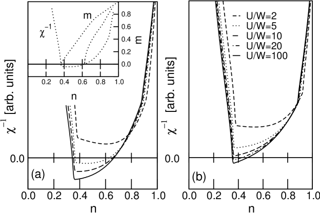
Figure 2: Inverse paramagnetic static susceptibility $\chi^{-1}$ for the sc lattice as a function of the band occupation n for various values of U. (a) System with the full $\vec{k}$-dependent selfenergy. (b) System with a local selfenergy ($F_{\vec{k}-\sigma}\equiv 0$). The inset shows the magnetic moment as a function of n for $U/W=5$.

Two important aspects of the SDA solution in Fig.2 should be stressed. The first concerns the comparison with the corresponding results of the Hubbard-I approach Hub63 , which does not allow ferromagnetism on the sc lattice. On the other hand, the Hubbard-I selfenergy differs from (35) “only” by neglecting the “band correction” $B_{\vec{k}-\sigma}$. Consequently, the stronger magnetic stability in the SDA must be due to $B_{\vec{k}-\sigma}$. The second remark aims at the non-locality ($\vec{k}$-dependence) of the electronic selfenergy provoked by the “bandwidth correction” $F_{\vec{k}-\sigma}$ (36) in $B_{\vec{k}-\sigma}$. Part (b) of Fig.2 demonstrates its importance. Switching off this term leads to a dramatic further increase of the critical coupling $\frac{U_{C}}{W}$ from 4 to 14. More detailed studies THerN97 , however, show that the influence of $F_{\vec{k}-\sigma}$ on magnetic stability strongly depends on the lattice type. Increasing coordination number $({\rm sc}\longrightarrow{\rm bcc}\longrightarrow{\rm fcc})$ drastically diminishes the importance of the non-locality leaving the local spin-dependent band shift $B_{-\sigma}$ as the pushing mechanism for ferromagnetic stability.

It can be shown HN97 that the SDA gives a qualitatively convincing picture of bandferromagnetism . The main message is that the spin-dependent “band-shift” $B_{-\sigma}$ and the lattice structure are the most important ingredients. However, we should not forget the disadvantages of the method. One of them is the neglect of quasiparticle damping, which is assumed to destabilize the collective spin order.

3.2 Quasiparticle Damping

More or less by construction the SDA selfenergy (35) is real except for a single $\delta$-peak in $Im\Sigma_{\vec{k}\sigma}(E+{\rm i}0^{+})$ at the pole $E=T_{0}+B_{\vec{k}-\sigma}+U(1-\langle n_{-\sigma}\rangle)-\mu$. It has, however, no influence since it falls into the Hubbard gap. The quasiparticles are stable. We are therefore looking for an approach that retains the obvious advantages of the SDA but improves it by a reasonable inclusion of quasiparticle lifetime effects.

Starting point is an alloy-analogy for the Hubbard model which traces back to Hubbard himself Hub64 . The idea is to consider the propagation of a $\sigma$ electron through the lattice with the $-\sigma$ electrons being “frozen” at their lattice sites and randomly distributed over the crystal. When the $\sigma$ electron enters a lattice site it can encounter two different situations. It can meet a $-\sigma$ electron or not. That can be interpreted as a hopping through a fictitious binary alloy, the two constituents of which are characterized by atomic levels $E_{1\sigma},E_{2\sigma}$ and by concentrations $x_{1\sigma},x_{2\sigma}$. The “coherent potential approximation” (CPA) is a standard method to perform the configurational average over the alloy VKE68 . The resulting $\sigma$ selfenergy obeys the following implicit equation NoltingBd7 ,

$$0=\sum\limits^{2}_{p=1}x_{p\sigma}\frac{E_{p\sigma}-\Sigma_{\sigma}(E)-T_{0}}{1-\frac{1}{\hbar}G_{\sigma}(E)(E_{p\sigma}-\Sigma_{\sigma}(E)-T_{0})}$$ (52)

$G_{\sigma}(E)=\frac{1}{N}\sum\limits_{\vec{k}}G_{\vec{k}\sigma}(E)$ is the local propagator. CPA is a single-site approximation, the resulting selfenergy therefore wave vector independent. To proceed one has to specify the two-component alloy. The natural way (“conventional alloy analogy” CAA) would be to use the zero-bandwidth results of the Hubbard model: $E_{1\sigma}=T_{0},E_{2\sigma}=T_{0}+U,x_{1\sigma}=1-\langle n_{-\sigma}\rangle=1-x_{2\sigma}$. The resulting $\Sigma_{\sigma}^{CAA}(E)$ includes quasiparticle damping but excludes any spontaneous ferromagnetism FE73 ; SD75 . Does quasiparticle damping really kill any spontaneous moment order? This is a serious question because it has been shown VV92 that for infinite lattice dimensions CPA is an exact (!) treatment of the alloy problem. On the other hand, the CAA selfenergy disagrees with the strong as well as weak coupling behaviour (24), (28). This discrepancy can only be removed by the conclusion that the zero-bandwidth limit constitutes the wrong alloy analogy HN96 .

The fictitious binary alloy is indeed by no means predetermined. We consider $E_{1,2\sigma}$ and $x_{1,2\sigma}$ at first as free parameters and fix them via the high-energy expansions (21) and (24), which we insert into the CPA equation (44). Then we expand eq. (44) with respect to powers of $\frac{1}{E}$. Comparing coefficients we can use the following set of equations to determine an “optimum alloy analogy”:

$$\sum\limits_{p=1}^{2}x_{p\sigma}=1$$ (53)

$$\sum\limits_{p=1}^{2}x_{p\sigma}(E_{p\sigma}-T_{0})=U\langle n_{-\sigma}\rangle$$ (54)

$$\sum\limits_{p=1}^{2}x_{p\sigma}(E_{p\sigma}-T_{0})^{2}=U^{2}\langle n_{-\sigma}\rangle$$ (55)

$$\sum\limits_{p=1}^{2}x_{p\sigma}(E_{p\sigma}-T_{0})^{3}=U^{3}\langle n_{-\sigma}\rangle+U^{2}B_{-\sigma}\langle n_{-\sigma}\rangle(1-\langle n_{-\sigma}\rangle)$$ (56)

Deriving from these equations $E_{p\sigma}$ and $x_{p\sigma}$ automatically guarantees the correct strong-coupling behaviour. One finds (p=1,2) (“modified alloy analogy” MAA).

$$E_{p\sigma}^{MAA}=$$ (57)

$$T_{0}+\frac{1}{2}[U+B_{-\sigma}+(-1)^{\cal P}\sqrt{(U+B_{-\sigma})^{2}-4\langle n_{-\sigma}\rangle B_{-\sigma}}]$$ (58)

$$\equiv(E_{p\sigma}^{SDA}(\vec{k}))_{\varepsilon(\vec{k})=T_{0}}\equiv f_{p}(T_{0},U,\langle n_{-\sigma}\rangle,B_{-\sigma})$$ (59)

$$x_{1\sigma}^{MAA}=\frac{B_{-\sigma}+T_{0}+U(1-\langle n_{-\sigma}\rangle)-E^{MAA}_{1\sigma}}{E_{2\sigma}^{MAA}-E_{1\sigma}^{MAA}}=1-x^{MAA}_{2\sigma}$$ (60)

$$x_{p\sigma}^{MAA}\equiv(\alpha^{SDA}_{p\sigma})_{\varepsilon(\vec{k})=T_{0}}\equiv g_{p}(T_{0},U,\langle n_{-\sigma}\rangle,B_{-\sigma})$$ (61)

Surprisingly, the energies and weights coincide exactly with the corresponding SDA entities if $\varepsilon(\vec{k})$ is simply replaced by $T_{0}$. Because of the single-site aspect of the CPA VKE68 ; NoltingBd7 the “band-correction” $B_{\vec{k}-\sigma}$ is restricted here to its local part $B_{-\sigma}$, the decisive band shift. Inserting (46) and (47) into (44) yields the MAA selfenergy for all E which exhibits some remarkable features HN96 :

• As a CPA result the MAA includes quasiparticle damping ($Im\Sigma_{\sigma}^{MAA}(E)\not=0$), and that without giving up the advantages of the SDA.

• The expectation values $\langle n_{-\sigma}\rangle$ and $B_{-\sigma}$ are to be determined selfconsistently. In principle, they take care for a carrier concentration-, temperature- and spin-dependence of the atomic data (46),(47) of the alloy constituents. Furthermore, and that is quite an important aspect, $B_{-\sigma}$ brings into play in a certain sense the itineracy of the $-\sigma$ electrons (“correlated” electron hopping), completely neglected in the CAA.

• Strong-coupling and high-energy behaviour are correctly reproduced, more or less by construction.

• The general CPA theory VKE68 comes for the so-called split-band regime (here, $U\gg W$) to the conclusion that the spectral density $S_{\vec{k}\sigma}(E)$ should consist of two separated peaks with centres at

  $$T_{\vec{p}\sigma}^{CPA}=E_{\vec{p}\sigma}+x_{\vec{p}\sigma}(\varepsilon(\vec{k})-T_{0});\qquad p=1,2$$ (62)

  Inserting (46) and (47) for $U\gg W$ yields exactly the Harris-Lange results (6-8), a further strong confirmation of the MAA.

• Contrary to the CAA the MAA allows for spontaneous bandferromagnetism.

For a typical example the possibilities of the MAA are demonstrated in Fig.3, which shows $S_{\vec{k}\sigma}(E)$ for strongly correlated electrons $(\frac{U}{W}=5)$ on an fcc lattice. For less than half-filled bands ($n<1$) the system is paramagnetic. The band occupation n=1.6 used in Fig.3 allows for a spontaneous collective order provided U exceeds a critcal value. Two types of splitting occur. At first the spectral density consists for each $\vec{k}$-vector of a high-energy and a low-energy peak separated by an energy of order U. The finite widths of the peaks are due to quasiparticle damping and obviously energy-, wave-vector-, spin- and temperature-dependent. The spectral weight (area) of the low-energy peak scales with the probability that the propagating ($\vec{k},\sigma$)-electron in the more than half-filled band enters an empty lattice site, the weight of the upper peak that it meets anywhere a $-\sigma$ electron. This splitting is general and not at all bound to ferromagnetism. It demonstrates the correct strong-coupling behaviour (6,7). Ferromagnetism appears when the two spectral density peaks show a spin asymmetry. For the low temperature example $T=100K$ (Fig.3a) the system is close to saturation ($m=2-n$), i.e. the up-spin states are almost fully occupied. A down-spin electron cannot avoid to meet an up-spin electron at every lattice site being therefore forced to perform a Coulomb interaction. Consequently the low-energy peak of $S_{\vec{k}\downarrow}(E)$ disappears. At higher temperatures (Fig.3b) the peak reappears because of a partial demagnetisation, i.e. a finite density of holes in the up-spin spectrum. At low temperatures the high-energy peaks of $S_{\vec{k}\downarrow}(E)$ are very sharp indicating long-living quasiparticles. A $\downarrow$-hole has no chance to meet an $\uparrow$-hole to be scattered.

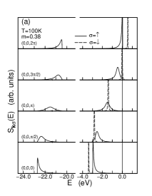
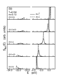
Figure 3: Spectral density as a function of energy for an fcc lattice calculated within the MAA, (a) $T=100K$, (b) $T=615K$ for different $\vec{k}$-vectors equidistant along the (001)-direction of the 1. Brillouin zone. Further parameters: $n=1.6,\quad U=20eV,\quad W=4eV$. The vertical line indicates the position of the chemical potential.

An interesting $\vec{k}$-dependence of the exchange splitting is observed. At the branch-top (X-point) a “normal” splitting apppears, i.e. the down-spin peak is above the up-spin peak. At the bottom ($\Gamma$-point), however, the $\uparrow$-peak is higher in energy than the $\downarrow$-peak (“inverse exchange splitting”). The quasiparticle dispersions of the two spin-parts are crossing as a function of $\vec{k}$. This behaviour is a result of two competing correlation effects. The one is the spin-dependent exchange shift of the centres of gravity of the quasiparticle subbands, the other a spin-dependent band narrowing. The latter may overcompensate the first. In any case the exchange splitting exhibits a strong wave-vector dependence, even with a sign change.

We can conclude that the MAA improves the SDA in a systematic manner by including quasiparticle damping. As will be discussed in Sect. 4, the main modification consists in a substantial destabilisation of ferromagnetism in the Hubbard model. One reason is the finite overlap of the spectral density peaks, in the SDA because of (34) excluded, which weakens the ferromagnetic solution of the selfconsistently evaluated model theory.

The second shortcoming of the SDA, the incorrect weak-coupling behaviour, persists in the MAA. In the following we have to inspect its consequences for the strong-coupling phenomenon ferromagnetism.

3.3 Weak-coupling behaviour

Neither the SDA selfenergy (35) nor the MAA selfenergy does fulfill the weak-coupling expansion (28). We are now looking for an approach which interpolates reasonably between the strong- and weak-coupling regimes. It should extend the preceding approaches SDA and MAA by inclusion of weak coupling and Fermi liquid behaviour without giving up the convincing essentials from the SDA and MAA: spin-dependent band shift $B_{-\sigma}$ and quasiparticle damping. Following an idea of Kajueter and Kotliar KK96 we start with a selfenergy ansatz PWN97 , which we call the “modified pertubation theory” (MPT):

$$\Sigma_{\vec{k}\sigma}(E)=U\langle n_{-\sigma}\rangle+\frac{a_{\vec{k}\sigma}U^{2}\Delta_{\vec{k}\sigma}(E)}{1-b_{\vec{k}\sigma}U^{2}\Delta_{\vec{k}\sigma}(E)}$$ (63)

The second order contribution $\Delta_{\vec{k}\sigma}(E)$ is defined in eq. (29). We use in $\Delta_{\vec{k}\sigma}(E)$ for the spectral densities the Hartree-Fock version (30) with the selfconsistency condition (31). By construction the selfenergy (49) is correct in the weak-coupling regime up to order $U^{2}$. In order to fulfill simultaneously the strong-coupling regime we expand (49) in powers of the inverse energy $1/E$ and compare this with the exact selfenergy expansion (24). The first two terms are automatically fulfilled, the third and the fourth fit the coefficients $a_{\vec{k}\sigma},\;b_{\vec{k}\sigma}$ PWN97 . For the results presented in the next section we have implemented the MPT (49) in a “dynamical mean field theory” (DMFT) procedure PWN97 ; WPN98 . The main assumption is then a local selfenergy $\Sigma_{\vec{k}\sigma}(E)\to\Sigma_{\sigma}(E)$ , exact in infinite lattice dimensions MV89 . Furthermore, we exploit the fact that the Hubbard problem can be mapped under such conditions on the single-impurity Anderson model (SIAM) (see contribution of D. Vollhardt ) as long as a special selfconsistency condition is fulfilled PWN97 . The idea of the MPT is then applied to the simpler SIAM problem. It can be shown, however, that the direct application of the MPT-concept to the Hubbard model gives almost the same results.

Figure 4: Curie temperature as a function of band “filling” (hole concentration) for an fcc-type $d=\infty$-lattice (51). The points with error bars are the Quantum-Monte-Carlo results from ref. [3]. SDA, MAA and MPT are explained in the text.

The MPT fulfills a maximum number of limiting cases: The weak-coupling behaviour is correct up to $U^{2}$-terms, for all bandoccupations $n$ Fermi liquid properties are recovered. The Luttinger theorem,

$$S_{ii\sigma}(0)\stackrel{{\scriptstyle!}}{{=}}S^{(0)}_{ii\sigma}(0)\;\leftrightarrow\;\mu=\mu|_{U=0}+\Sigma_{\sigma}(0)\;,$$ (64)

is fulfilled for all bandoccupations $n$, at least if not too far from half-filling ($n=1$). For low temperatures a Kondo resonance appears at the chemical potential $\mu$. The zero-bandwidth limit ($W\to 0$) comes out exact for all $n$ as well as the strong-coupling behaviour gathered in eqs. (6)-(8). Eventually bandferromagnetism is possible within the framework of MPT. According to the number of correctly reproduced limiting cases the MPT appears to be an optimum approach to the many-body problem of the Hubbard model.

4 Discussion

Let us compare the analytical approaches presented in the preceding Section with respect to the most important magnetic key-quantity, the Curie temperature $T_{\rm C}$. For comparison with the numerically essentially exact Quantum Monte Carlo results of Ulmke Ul98 we have evaluated the three theories for an fcc-$d=\infty$ type lattice described by the Bloch density of states:

$$\rho_{0}(E)=\frac{\exp{\big{(}-\frac{1}{2}(1-\frac{\sqrt{2}E}{t^{\ast}})\big{)}}}{t^{\ast}\sqrt{\pi(1-\frac{\sqrt{2}E}{t^{\ast}})}}$$ (65)

The energy unit is chosen to $t^{\ast}=t\sqrt{2d(d-1)}\stackrel{{\scriptstyle!}}{{=}}1$. The density of states (51) is strongly asymetric with a square root divergency at the upper edge.

All the presented methods predict that ferromagnetism exists only for more than half-filled energy bands. In Fig. 4 bandfilling therefore means the hole-density and the DOS is that for holes following from (51) by $t^{\ast}\to-t^{\ast}$.

Figure 5: Left: Quasiparticle density of states as function of energy for the fcc-type lattice (51). Solid lines for $\sigma=\uparrow$, dotted lines for $\sigma=\downarrow$. QMC results from [3]. Temperature T is chosen so that for all presented methods a magnetization $\rm{m}=0.4$ is found. Right: For the same parameters as in the left part the magnetisation m and the inverse paramagnetic susceptibility $\chi^{-1}$ as function of the reduced temperature $T/T_{\rm{C}}$. Bottom figure: QMC results, dashed line for $T/T_{\rm{C}}\leq 1:S=1/2$-Brillouin function.

The role of the spin-dependent band shift $B_{-\sigma}$ (10) for the magnetic stability becomes evident by comparison of the three methods with their $B_{-\sigma}=0$ counterparts. That is for SDA the Hubbard I-solution Hub63 which yields ferromagnetism only for very asymmetric DOS. In the case of (51) there appears ferromagnetism in a strongly restricted region of very low hole densities. The band shift $B_{-\sigma}$ in the SDA obviously leads to a drastic enhancement of ferromagnetic stability. The counterpart of MAA is the conventional alloy analogy (CAA) that does not allow for any $n$ ferromagnetic order FE73 ; SD75 . Finally, the MPT-counterpart, that neglects the bandshift, is the Kajueter-Kotliar approach KK96 . It indeed exhibits ferromagnetism but with substantially lower Curie temperatures $T_{\rm C}$.

The influence of quasiparticle damping can best be judged by comparing the results of SDA and MAA. The inclusion of lifetime effects in MAA presses the Curie temperature to half the SDA-values. The ferromagnetic coupling strength is therefore substantially weakened by quasiparticle damping. The incorporation of the correct weak-coupling behaviour by MPT leads to a further $T_{\rm C}$-reduction possibly because of the screening tendency with respect to the effective magnetic moments manifesting itself in the appearance of a Kondo resonance. The MPT-results for $T_{\rm C}(n)$ are closest to the essentially exact numerical results of Ulmke Ul98 , which have been read off from the zeros of the inverse paramagnetic susceptibility.

The similarities and the differences of the various methods come out by the quasiparticle density of states in Fig. 5a. All theories show the splitting into the two Hubbard bands and the additional exchange splitting which takes care for the spin asymmetry. As a consequence of the neglect of damping effects the DOS-structures are rather sharp in the SDA. They appear smoother in MAA. The correct low-energy behaviour of the MPT leads to the best approach to the Q-DOS found by “Quantum Monte Carlo” (QMC)-evaluation of a “Dynamical Mean Field Theory”. Note that for a reasonable comparison of the Q-DOS we have chosen in Fig. 5a for the various theories temperatures which lead to the same magnetization $m=0.4$.

Fig. 5b demonstrates impressively the qualitative equivalence of the presented methods when we plot the spontaneous magnetization and the paramagnetic susceptibility as function of the reduced temperature $T/T_{\rm C}$. There are indeed strong similarities. All magnetization curves are Brillouin function-like with full polarization at $T=0$. The only exception is MPT, which shows up a slight deviation from saturation at $T=0$. For the chosen parameter set all methods predict a second order transition at $T_{\rm C}$. The paramagnetic susceptibility follows in all theories a ideal Curie-Weiß behaviour: $\chi=C(T-\Theta)^{-1}$. The paramagnetic Curie temperature $\Theta$ equals in any case the Curie temperature $T_{\rm C}$ and even the Curie constants $C$ are all very similar: $C=$0.42 (SDA), 0.52 (MAA), 0.57 (MPT), 0.47 (QMC). One important consequence of this striking qualitative equivalence and correctness of SDA, MAA and MPT compared to QMC is that even the rather simple SDA can be used to describe the magnetism of more complicated structures (films, surfaces, multilayer, real substances).

We conclude that ferromagnetism does exist in the Hubbard model depending on lattice structure, band occupation, Coulomb coupling and temperature. By a critical comparison of three different analytical approaches we could demonstrate the essentials for ferromagnetic stability, in a positive sense the spin-dependent band shift $B_{-\sigma}$, which represents the correlated hopping of opposite spin electrons, and in a negative sense the finite lifetime of quasiparticles, which results in a drastic lowering of the ferromagnetic coupling strength. The correct inclusion of Fermi liquid properties eventually leads to the most convincing description of ferromagnetism in the Hubbard model.

References

- (1) H. Capellmann: ‘Metallic Magnetism’. Vol. 42 of: Springer Topics in Current Physics, (Springer, Berlin 1987).
- (2) Y. Nagaoka: Phys. Rev. 147, 392 (1966).
- (3) M. Ulmke: Eur. Phys. J. B 1, 301 (1998).
- (4) W. Metzner, D. Vollhardt: Phys. Rev. Lett. 62, 324 (1989).
- (5) E. Müller-Hartmann: Z. Phys. B 74, 507 (1989).
- (6) G. D. Mahan, ‘Many Particle Physics’, Vol. 42, (Plenum Press, New York 1990).
- (7) A. B. Harris, R. Lange: Phys. Rev. 157, 295 (1967).
- (8) G. Geipel, W. Nolting: Phys. Rev. B 38, 2608 (1988).
- (9) W. Nolting, W. Borgieł: Phys. Rev. B 39, 6962 (1989).
- (10) J. Hubbard: Proc. Roy. Soc. A276, 238 (1963).
- (11) W. Nolting: ‘Vielteilchentheorie’. Bd. 7 of: Grundkurs: Theoretische Physik. (Vieweg, Wiesbaden 1997).
- (12) A. A. Abrikosov, L. P. Gorkov, I. E. Dzyaloshinsky: ‘Methods of Quantum Field Theory in Statistical Physics’. (Prentice Hall, New Jersey 1964).
- (13) H. Schweitzer, G. Czycholl: Solid State Commun. 74, 735 (1990).
- (14) V. Zlatic, B. Horvatic: Phys. Rev. B 28, 6904 (1983).
- (15) H. Kajueter, G. Kotliar: Phys. Rev. Lett. 77, 131 (1996).
- (16) J. M. Luttinger: Phys. Rev. 121, 942 (1961).
- (17) T. Herrmann, W. Nolting: J. Magn. Magn. Mater. 170, 253 (1997).
- (18) L. M. Roth: Phys. Rev. 184, 451 (1969).
- (19) T. Herrmann, W. Nolting: Solid State Commun. 103, 351 (1997).
- (20) J. Hubbard: Proc. Roy. Soc. A281, 401 (1964).
- (21) B. Velický, S. Kirkpatrick, H. Ehrenreich: Phys. Rev. 175, 747 (1968).
- (22) H. Fukuyama, H. Ehrenreich: Phys. Rev. B 7, 3266 (1973).
- (23) J. Schneider, V. Drchal: phys. stat. sol. (b) 68, 207 (1975).
- (24) R. Vlaming, D. Vollhardt: Phys. Rev. B 45, 4637 (1992).
- (25) T. Herrmann, W. Nolting: Phys. Rev. B 53, 10579 (1996).
- (26) M. Potthoff, T. Wegner, W. Nolting: Phys. Rev. B 50, 16132 (1997).
- (27) T. Wegner, M. Potthoff, W. Nolting: Phys. Rev. B 57, 6211 (1998).