Interacting fermions in self-similar potentials

Abstract

We consider interacting spinless fermions in one dimension embedded in self-similar quasiperiodic potentials. We examine generalizations of the Fibonacci potential known as precious mean potentials. Using a bosonization technique and a renormalization group analysis, we study the low-energy physics of the system. We show that it undergoes a metal-insulator transition for any filling factor, with a critical interaction that strongly depends on the position of the Fermi level in the Fourier spectrum of the potential. For some positions of the Fermi level the metal-insulator transition occurs at the non interacting point. The repulsive side is an insulator with a gapped spectrum whereas in the attractive side the spectrum is gapless and the properties of the system are described by a Luttinger liquid. We compute the transport properties and give the characteristic exponents associated to the frequency and temperature dependence of the conductivity.

I Introduction

The electronic properties of quasicrystalsshechtman_quasi_discovery have revealed the importance of the non crystalline order at the atomic level. Indeed, the conductivity $\sigma$ of these metallic alloys displays a unusual behavior since it increases when either temperature or disorder increases. It is also surprisingly low compared to that of the metals that composed them. From a theoretical point of view, the influence of quasiperiodicity on the spectral and dynamical properties of electron systems has been the subject of many studiesSire_aussois ; schulzbaldes_aperiodic_transport ; piechon_diffusion_fibo ; sire_quasi_gaps ; ketzmerick_quasi_wavepacket ; roche_review_quasi . For independent electrons systems, it has been shown that the eigenstates, which are neither localized nor extended but critical (algebraic decay), are responsible of an anomalous quantum diffusion in any dimension. Concerning the nature of the spectrum, it depends on the dimensionality but also exhibits specific characteristics of the quasiperiodicity. More precisely, in one dimension, the spectrum of quasiperiodic systems, such as the Fibonacci or the Harper chain, is made up of an infinite number of zero width bands (singular continuous) whereas in higher dimensions, it can be either absolutely continuous (band-like), singular continuous, or any mixture. These features are a direct consequence of the long-range order present in these structures despite the lack of periodicity. This absence of translational invariance makes any analytical approach difficult and one must often have recourse to numerical diagonalization, except in a perturbative frameworksire_quasi_gaps ; piechon_diffusion_fibo .

Given the complexity of the independent electron problem, the influence of a quasiperiodic modulation on an interacting system is very difficult to tackle. Attempts to solve this problem have been mostly confined to mean field solutionshiramoto_hartreefock_quasi or numerical diagonalizations chaves_meso_transport ; chaves_harper_meanfield ; eilmes_mit_twoparticles . We have recently proposed vidal_quasi_interactions_short a different route, already used with success for periodic giamarchi_umklapp_1d ; giamarchi_mott_shortrev and disordered systemsapel_spinless ; giamarchi_loc . The main idea of this method is to first solve the periodic system in presence of interactions ; this is relatively easy, either in the one-dimensional case for which technique to treat interactions existssolyom_revue_1d ; emery_revue_1d ; schulz_houches_revue ; voit_bosonization_revue , or even in higher dimensions through approximate (Fermi liquid) solutions. In a second step, we study the effect of a perturbative quasiperiodic potential via a renormalization group approach. Several types of quasiperiodic potentials can in principle be studied by this approach but the most interesting effects come from quasiperiodic potentials which have a non trivial Fourier spectrum. Indeed other potentials such as the Harper modelkolomeisky_harper_perturbatif ; sen_quasi_dimerization ; sen_quasi_renormalization who have only a single harmonic in their Fourier spectrum are perturbatively equivalent to periodic systems giamarchi_umklapp_1d . We have used our RG approach to treat interacting spinless fermions in the presence of a Fibonacci potentialvidal_quasi_interactions_short ; vidal_quasiinter_mbx . We have shown that the existence of arbitrarily small peaks in the Fourier spectrum (opening arbitrarily small gaps at first order in perturbation) leads to a vanishing critical interaction below which the system is conducting. This novel metal-insulator transition (MIT) has very different characteristics from those observed in periodic and disordered systems for which a finite attractive interaction is required. These predictions have been successfully confirmed by numerical calculationsHida_quasi_spinless_DMRG ; Hida_precious . Similar renormalization techniques have been also used in a variety of cases mastropietro_quasi_smalldenominators ; sen_quasi_dimerization ; sen_quasi_renormalization ; Hida_quasi_spinfull . Even if some of these properties are specific to one-dimensional potentials, these results should provide a first step toward the understanding of higher dimensional interacting system in quasiperiodic structures.

In the present paper, we extend this study to quasiperiodic potentials that generalize the Fibonacci potential. We show that the critical properties obtained in the Fibonacci casevidal_quasi_interactions_short are generic of other self-similar systems. Our results are in agreement with the recent numerical results obtained on precious mean potentialsHida_precious . The paper is organized as follows : in Section II, we present the model on the lattice and derive its continuous version for any potential using a bosonization technique. We detail the renormalization group treatment of the bosonized model and the computation of the flow equations for the coupling constants. In Section III, we recall the results for the well-known Mott transition (periodic case) and we describe the physics of the disordered case for which a different kind of MIT occurs. We then discuss the most interesting situation : the quasiperiodic case. We explain why the non trivial self-similar Fourier spectrum induces a MIT whose characteristics are intermediate between the periodic and the disordered potentials. The physical consequences are discussed in the Section IV with a special emphasis on the transport properties. We also discuss the question of the strong coupling regime. Conclusions can be found in Section V and some technical details are given in the appendices.

II Description of the Model and Renormalization

II.1 The Model

We consider a system of interacting spinless fermions in a one-dimensional lattice of linear size $La$ ($a=1$ being the lattice spacing) described by the following Hamiltonian :

$$H = -t\sum_{i}c^{\dagger}_{i+1}\,c_{i}+c^{\dagger}_{i}\,c_{i+1}+$$ (1)

$$V\sum_{i}n_{i}\,n_{i+1}+\sum_{i}W_{i}\,n_{i}$$

$$= H_{t}+H_{V}+H_{W}$$ (2)

where $c^{\dagger}_{i}$ (resp. $c_{i}$) denotes the creation (resp. annihilation) fermion operator, $n_{i}=c^{\dagger}_{i}\,c_{i}$ represents the fermion density on site $i$. In (1), $t$ represents the hopping integral between sites and $V$ controls the strength of the interaction between nearest-neighbor particles. In addition, the fermions are embedded in an on-site (diagonal) potential $W$. In the following, we consider three main categories for $W$ : $(i)$ a simple periodic potential of the form $W_{i}=\lambda\cos(Qi)$; $(ii)$ a random potential uncorrelated from site to site; $(iii)$ a quasiperiodic potential whose study is the aim of this paper. In this latter case, we will focus on the general class of precious mean potentials described in Appendix A.

In order to treat the interactions in (1), it is convenient to write the fermion operators in term of boson ones. This bosonization techniquesolyom_revue_1d ; emery_revue_1d ; schulz_houches_revue ; voit_bosonization_revue provides a good description of the low-energy physics of the Hamiltonian $H_{0}(t,V)=H_{t}+H_{V}$. For completeness and to fix the notations we give a brief summary of this method in Appendix B. Within this framework, $H_{0}(t,V)$ can be rewritten :

$$H_{0}(t,V)={1\over 2\pi}\int dx\>(uK)(\pi\Pi)^{2}+\left({u\over K}\right)(\partial_{x}\phi)^{2}\mbox{,}$$ (3)

where $\phi$ and $\Pi$ are conjugate bosonic fields respectively related to the long wavelength part of the density and the current (see Appendix B). All interaction effects can be absorbed in the so-called Luttinger liquid parameters : $u$, the velocity of the charge excitations, and $K$ which controls the behaviour of the various correlation functions (see below). For $V\ll t$, analytic expressions of these parameters can be obtained (see (93-94)). However, the bosonic representation is in fact quite general and the expression (3) provides the effective Hamiltonian describing the low-energy physics of any one-dimensional interacting spinless fermionic system haldane_xxzchain ; haldane_bosonisation .

Concerning the coupling to the lattice potential $W$, one has, in the continuum limit (see Appendix B) :

$$H_{W} = \int dx\>W(x)\,\rho(x)$$ (5)

$$= \int dx\>W(x)\times$$

$$\left(-{1\over\pi}\partial_{x}\phi(x)+{1\over\pi\alpha}\cos(2\phi(x)-2k_{F}x)\right)\mbox{.}$$

The various physical observables can be expressed in terms of the boson fields. For example, the correlation function of the $2k_{F}$ part of the density is :

$$R(x,\tau,x^{\prime},\tau^{\prime}) = \left\langle T_{\tau}\rho_{2k_{F}}(x,\tau)\>\rho_{2k_{F}}(x^{\prime},\tau^{\prime})\right\rangle$$ (6)

$$\sim \left\langle T_{\tau}e^{i2\phi(x,\tau)}e^{-i2\phi(x^{\prime},\tau^{\prime})}\right\rangle\mbox{,}$$ (7)

where $T_{\tau}$ is the time-ordering operator for the imaginary time $\tau$. In absence of the perturbation $H_{W}$, one has :

$$R(x,\tau,x^{\prime},\tau^{\prime})\sim\left({\alpha\over|{\bf r-r^{\prime}}|}\right)^{2K}\hbox{for}\ \ |{\bf r-r^{\prime}}|\gg\alpha\mbox{,}$$ (8)

where ${\bf r}=(x,\tau)$.

II.2 Renormalization Group Analyzis

To study the influence of the potential $W$, we use a standard RG approach by analyzing perturbatively the renormalization of the correlation function (7) computed with the full action of the system. First, note that via a redefinition of the bosonic field $\phi$ :

$$\tilde{\phi}(x)=\phi(x)-{K\over u}\int^{x}dy\,W(y)\mbox{,}$$ (9)

the term proportional to $\partial_{x}\phi$ in (5) can be absorbed in the quadratic part of the action which thus writes :

$$S_{0}={1\over 2\pi}\int d{\bf r}\>\left[{1\over uK}(\partial_{\tau}\tilde{\phi})^{2}+\left({u\over K}\right)(\partial_{x}\tilde{\phi})^{2}\right]\mbox{.}$$ (10)

Introducing the Fourier components by :

$$W(x)=\lambda\,\sum_{Q}{\hat{W}(Q)}e^{iQx}\mbox{ , }$$ (11)

the potential part of the action reads :

$$S_{W} = {g\over u(2\pi\alpha)^{2}}\sum_{Q}{\hat{W}(Q)}\times$$

$$\int d{\bf r}\>e^{i\left(2\phi(x,\tau)+Q^{-}x\right)}+e^{i\left(-2\phi(x,\tau)+Q^{+}x\right)}\mbox{,}$$

where $Q^{\pm}=Q\pm 2k_{F}$ and $g=2\pi\alpha\lambda$. Treating $S_{W}$ perturbatively and imposing that the asymptotic behavior (8) is unchanged when varying the cut-off $\alpha$ leads to the renormalization of the parameter $K$ and of the Fourier components of the potential $W$. The procedure is detailed in Appendix C. The RG equations are given by :

$${dK\over dl} = -K^{2}\,\Xi(l)\mbox{,}$$ (13)

$${dy_{Q}\over dl} = (2-K)\,y_{Q}\mbox{,}$$ (14)

with :

$$\Xi(l)={1\over 2}\sum_{Q}y_{Q}^{2}\left[\mbox{J}(Q^{+}\alpha(l))+\mbox{J}(Q^{-}\alpha(l))\right]\mbox{,}$$ (15)

where the $y_{Q}=\lambda\alpha\hat{W}(Q)/u$ are the dimensionless Fourier components of $W$ and $l$ is the scale factor defined by $\alpha(l)=\alpha(0)e^{l}$ where $\alpha(0)=\alpha$ is proportional to the original lattice spacing $a$. In (15), J is a function whose precise form depends on the cut-off procedure used to eliminate the short distance degrees of freedom (see Appendix C). Different kind of functions are considered below, but one typically has :

$$\mbox{J}(Q^{\pm}\alpha(l)) \simeq 1\>\>\mbox{for}\>\>\alpha(l)<1/Q^{\pm}$$ (16)

$$= 0\>\>\mbox{otherwise}\mbox{.}$$ (17)

Physically, this means that the renormalization is equivalent to an investigation of the low-energy properties in a window around $2k_{F}$ in the reciprocal space whose width is proportional to $e^{-l}$. Thus, the full Fourier landscape of the potential determines the scaling of the parameters $K$ and $y_{Q}$. This is summarized in Fig. 1.

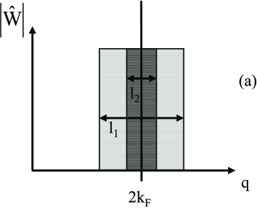
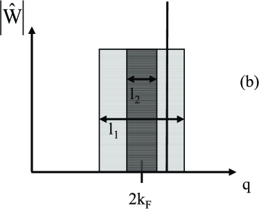
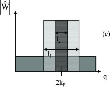
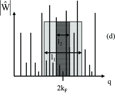
Figure 1: Schematic view of the renormalization procedure. The function $J$ (see text) filters the Fourier components $\hat{W}(q)$ of the potential and only keep those in a narrowing window around the Fermi level (i. e. for $q=2k_{F}$) as the scale increases. We have displayed the windows for two different scales $l_{1}$ and $l_{2}>l_{1}$. For the periodic case the potential has only one peak. If the potential is commensurate with $2k_{F}$ (a), the peak is inside the windows at all scales and the renormalization never stops. If the potential is incommensurate (b) it only acts if the peak remains in the windows (which is the case for $l_{1}$ but not at the larger scale $l_{2}$). For the disorder (c) case the potential has component at all $q$ thus the strength of the potential efficient in the renormalization is directly proportional to the size of the window. For the quasiperiodic case (d) the potential has a complicated peaks structure that gives rise to a novel behavior for the MIT.

III Critical properties

In this section, we discuss the relevance of the interactions for different potentials. In other words, we analyze the possibility of phase transition when varying the strength of the interactions.

III.1 Periodic potentials

This is the simplest case since the potential involves only one harmonic :

$$W(x)=\lambda\cos(Q\,x)\mbox{.}$$ (18)

Inserting the form (18) in (13-14) leads to the following flow equations giamarchi_umklapp_1d  :

$${dK\over dl} = -K^{2}y^{2}\left[\mbox{J}(Q^{+}\alpha(l))+\mbox{J}(Q^{-}\alpha(l))\right]\mbox{,}$$ (19)

$${dy\over dl} = (2-K)y\mbox{,}$$ (20)

where $y=\lambda\alpha/u$. Two different behaviors have to be distinguished depending on whether $\pm Q$ coincides with $2k_{F}$ or not.

III.1.1 Incommensurate case ($Q^{+}\neq 0$ and $Q^{-}\neq 0$)

In this case, there always exists a scale $l^{*}$ such that $\mbox{J}(Q^{\pm}\alpha(l^{*}))=0$, as shown on Fig. 1. At this scale the renomalization of $K$ essentially stops. $K$ thus converges towards a fixed point $K^{*}$, and the potential $W$ is irrelevant. The system remains a Luttinger liquid with gapless excitationsgiamarchi_umklapp_1d ; giamarchi_mott_shortrev and the correlation functions decay with an effective exponent $K^{*}$. This can be understood by the fact that, in this case, the Fermi level does not lie in the gap opened by the periodic potential $W$.

III.1.2 Commensurate case ($Q^{+}=0$ or $Q^{-}=0$)

Suppose for instance that $Q=2k_{F}$. In that case $\mbox{J}(Q^{-}\alpha(l))=1$ at all scales and the renormalization of $K$ cannot be stopped, as shown on Fig. 1. The potential is commensurate and would, for non interacting electrons ($K=1$) open a gap at the Fermi level. For interacting particles, the effect of the potential is given by the flow (19-20) which is now a simple Beresinskii-Kosterlitz-Thouless flow Berezinskii1 ; Berezinskii2 ; kosterlitz_modele_xy . Thus, for $K>2$, the potential $W$ is irrelevant, and the system remains a gapless Luttinger liquid. For $K<2$, the potential is relevant and the system flows to strong coupling regime. The strong coupling fixed point is not reachable by the perturbative flow but, since the system is described in this case by a simple sine-Gordon action, we know, from other methods, the physical properties of this phase emery_revue_1d ; schulz_houches_revue ; voit_bosonization_revue . A gap opens in the spectrum between the ground state and the first excited state. An estimate for this gap can be obtained from the RG analysis. If $l^{*}$ denotes the lengthscale at which $y\sim 1$, the gap is given by :

$$\Delta\propto e^{-l^{*}}\mbox{.}$$ (21)

In the case where $y\ll(2-K)$ one can neglect the renormalization of $K$ in (20) and we obtain :

$$\Delta\sim y^{1\over 2-K}\mbox{.}$$ (22)

Note that for the non interacting point ($K=1$), one recovers the linear scaling of $\Delta$ with respect to the strength of the potential $\lambda$ expected by the first order perturbation theory. This MIT induced by the interaction is known as the Mott transition. Let us emphasize that this critical value $K_{c}=2$, separating a metallic phase $(K>K_{c})$ from an insulating one $(K<K_{c})$, corresponds to attractive interactions between fermions.

The later discussion on the single harmonic case still holds for a potential with a finite number of Fourier components. The possibility of an insulating regime is then offered when the Fermi level is in one of the gaps opened by the various frequencies of the potential. The most interesting situation thus arises when the Fourier spectrum of the potential is dense or continuous. Such potentials can be encountered in several physical systems but we focus here on two of them : the random and the quasiperiodic potentials.

III.2 Disordered potentials

Let us consider a potential provided by a random variable with uniform probability whose Fourier components satisfy :

$$\overline{\hat{W}^{*}(Q)\hat{W}(Q^{\prime})}=\lambda\,\delta_{QQ^{\prime}}\mbox{.}$$ (23)

Using the general expressions (13) and (14) one obtains :

$${dK\over dl} = -{K^{2}\,y^{2}\over 2}\sum_{Q}\left[\mbox{J}(Q^{+}\alpha(l))+\mbox{J}(Q^{-}\alpha(l))\right]\mbox{,}$$ (24)

$${dy\over dl} = (2-K)\,y\mbox{.}$$ (25)

In Eq. (24), the sum actually stands for an integral so one has :

$$\sum_{Q}\left[\mbox{J}(Q^{+}\alpha(l))+\mbox{J}(Q^{-}\alpha(l))\right]\rightarrow\int dQ\left[\mbox{J}(Q^{+}\alpha(l))+\mbox{J}(Q^{-}\alpha(l))\right]\sim{1\over\alpha(l)}\sim e^{-l}\mbox{.}$$ (26)

This means that the renormalization of $K$ is directly proportionnal to the window width around $2k_{F}$ at scale $l$. In the limit of weak disorder the RG equations $(\ref{K_dis}-\ref{y_dis})$ can be integrated neglecting the renormalization of $K$ : $y(l)=y(0)\ e^{(2-K)\,l}$. One then has :

$${dK\over dl}=-CK^{2}e^{(3-2K)\,l}\mbox{,}$$ (27)

where $C$ is a constant. One deduces the existence of a critical point at $K_{c}=3/2$. Our approach thus generalises the RG treatment specific to the disorder case apel_spinless ; giamarchi_loc . For $K<K_{c}$, the system is insulating for any filling whereas it can be metallic for sufficiently attractive interaction. Note that for $K=1$, the system is an insulator as expected for a one-dimensional disordered non interacting system. By contrast to the periodic case, this transition point is independent of $k_{F}$. Physically, this can be understood invoking the proximity of several localized states (for $K=1$) at arbitrarily short distance that can couple to each other if the interaction is attractive enough. It is interesting to remark that the critical value in the disordered case ($K_{c}=3/2$) is smaller than in the periodic case ($K_{c}=2$). This means that the localization induced by the disorder is more easily destroyed by attractive interactions than the one induced by a finite width gap. In this context, it is clear that dense Fourier spectrum are able to provide rich outstanding situations where the position of the Fermi level could, in principle, determine the value of a critical point.

III.3 Quasiperiodic Potentials

To analyze such situations, we consider quasiperiodic potentials. Several types of potentials can play this role but, as already explained, the most interesting ones are those that have a non trivial dense Fourier spectrum. Here, we focus on quasiperiodic potentials obtained by substitution rules which lead to quasiperiodic effects even at the perturbative level. Among all possible choices, we consider the simplest one, known as precious mean potentials, that are given by the following iterative scheme :

$$A\rightarrow A^{k}B,\hskip 8.61108ptB\rightarrow A\mbox{.}$$ (28)

We associate, to each site, a diagonal potential that can take two discrete values $W_{A}=+\lambda/2$ or $W_{B}=-\lambda/2$. Let us note that a global shift of the $W_{i}$ always allows to deal with a zero-averaged potential so that we can set $\hat{W}(0)=0$. For $k=1$, one recovers the famous Fibonacci chain associated to the Golden Mean, for $k=2$ one has the Silver Mean sequence, etc. We give in the Appendix A a brief description of these sequences and a detailed calculation of their Fourier tranform. As it can be inferred from Fig. 2 ($k=1$) and Fig. 3 ($k=2$), the Fourier spectrum is dense in $[0,2\pi]$ in the quasiperiodic limit, and has a multifractal structure Peyriere .

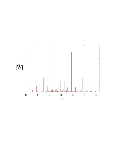
Figure 2: Fourier transform of the $15^{th}$ approximant of the Golden Mean (Fibonacci) potential (610 sites per unit cell).

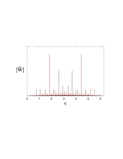
Figure 3: Fourier transform of the $10^{th}$ approximant of the Silver Mean potential (1393 sites per unit cell).

As in the periodic case, we have to consider several situations since we expect a strong dependence of the physical properties with respect to the position of the Fermi level. It is clear that if there exists a wave vector $Q\simeq 2k_{F}$ such that $\hat{W}(Q)$ is large compared to the other Fourier components, the electrons behave as if they were embedded in a periodic potential, whereas in the opposite case, i. e. the Fermi level lies in a very small gap, one could expect another behavior. Of course, the notion of far or close from a gap has only a sense once we have specified the maximum scale $l_{max}$ up to which we study the RG equations. In our case, since we only consider approximant (arbitrarily large), $\alpha(l_{max})$ is given by the inverse of the typical distance between gaps. Beyond this scale, the RG flow is no more sensitive to the precise structure of the Fourier spectrum. One can then encounter three situations :

III.3.1 $\hat{W}(2k_{F})$ is large

There is an harmonic of $W$ at $Q\simeq 2k_{F}$ such that $\hat{W}(2k_{F})$ is large compared to the other Fourier components. In other words, $\hat{W}(Q)$ opens a finite gap that dominates the low-energy physics up to a scale given by $(Q-2k_{F})^{-1}$. The function $\Xi$ that governs the flow of $K$ is then completely dominated by this component and behaves as $e^{(4-2K)\,l}$ (see Fig. 4). This actually defines the proximity of a “dominant” peak.

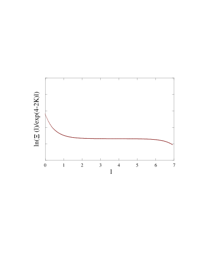
Figure 4: Behavior of $\Xi$ when the Fermi level $2k_{F}=2.4$ is close to a dominant peak (Fibonacci potential).

In this case, one recovers a critical value $K_{c}=2$ corresponding to that obtained in the periodic case, separating a metallic phase ($K>2$) from a insulating one ($K<2$).

III.3.2 $\hat{W}(2k_{F})$ is small

The Fermi level lies far from the main gaps. An example of such a situation is obtained at half filling $(2k_{F}=\pi)$. In this case, as shown in Fig. 5, $\Xi(l)\sim e^{(4-2K-2)\,l}$ for any kind of regulator.

Of course, this is not strictly speaking an exponential decrease and there is, in particular, some oscillations (in log-log) that are reminiscent of the multifractality of the Fourier spectrum. However, one can fairly approximates $\Xi(l)$ by $e^{2(1-K)\,l}$ and we obtain a critical point at $K_{c}=1$. This critical value corresponds to the non interacting point $V=0$. This means that when the Fermi level lies in zero width gap (small peaks) the slightest attractive interaction allows the system to become metallic whereas it is insulating at $V=0$. From a spectral point of view, this means that an attractive interaction close the gap and allows for arbitrarily low-energy excitations. This point will be discussed more in Sec. IV.2. We would like to stress that other positions of the Fermi level ($2k_{F}=0.5$ for Fibonacci for example) also gives $K_{c}=1$, and that similar situations occurs for other precious mean potentials (see Fig.6).

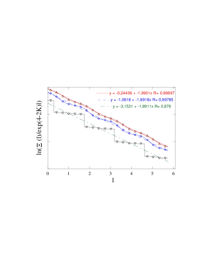
Figure 5: Behavior of $\Xi$ at half-filling ($2k_{F}=\pi$) for the Fibonacci potential. We have displayed the results for three different regulating function J : $\mbox{J}(x)=e^{-x^{2}}$$(\bigtriangleup)$, $\mbox{J}(x)=1/(1+x^{6})$ $(\diamond)$ and the step function $\mbox{J}(x)=1$ if $x<1$, 0 otherwise $(\bigtriangledown)$.

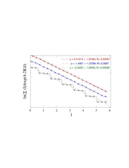
Figure 6: Behavior of $\Xi$ at half-filling ($2k_{F}=\pi$) for the silver mean potential. We have displayed the result for three different regulating function J : $\mbox{J}(x)=e^{-x^{2}}$$(\bigtriangleup)$, $\mbox{J}(x)=1/(1+x^{6})$ $(\diamond)$ and the step function $\mbox{J}(x)=1$ if $x<1$, 0 otherwise $(\bigtriangledown)$.

III.3.3 $\hat{W}(2k_{F})$ is intermediate

Finally, there are intermediate situations for which $\Xi(l)$ does not have an exponential behavior, even approximately. In these cases, it is impossible to simply extract a critical exponent and one needs a non perturbative treatment of the problem to determine a possible transition point (see Fig. 7). Note that in this case, one still observes the oscillations.

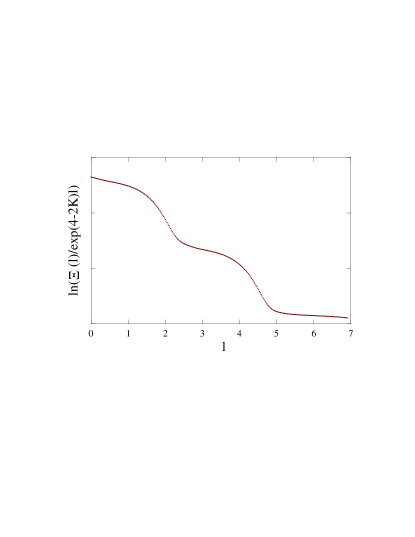
Figure 7: Behavior of $\Xi$ when the Fermi level $2k_{F}=0.5$ (Fibonacci potential) is in an intermediate situation.

IV Physical consequences

In addition to the phase diagram and the critical properties, determined in the previous section, the RG allows to extract many physical properties. In the metallic regime $K>K_{c}$ (where $K_{c}=2$ for periodic potential, $K_{c}=3/2$ for disordered potentials and $K_{c}=1$ for special filling factor in quasiperiodic potential), the system flows to weak coupling so the RG can be used at arbitrary scales. For the insulating side $K<K_{c}$ the potential flows to strong coupling. One can thus use the RG to obtain the properties up to the lengthscale $l^{*}$ such that the potential at this lengthscale is of order one. The behavior beyond this lengthscale (or below the correponding energy scale) can not be accessible by the RG and should be treated by other (non perturbative) methods. This point will be discussed in Sec. IV.2.

IV.1 Transport properties

Both the d. c. and a. c. transport properties of the system can in principle be extracted from the Kubo formula. The fermionic current operator can easily be written using the bosonic variables and reads :

$$j = v_{F}(\psi_{R}^{\dagger}\psi_{R}-\psi_{L}^{\dagger}\psi_{L})$$ (29)

$$= uK\Pi=\partial_{\tau}\phi\mbox{.}$$ (30)

Thus the conductivity is simply given by the correlation function :

$$\sigma(\omega)=\frac{i}{\omega}\left[\frac{2uK}{\pi}+\chi(\omega)\right]\mbox{.}$$ (31)

$\chi(\omega)$ is the retarded current-current correlation function :

$$\chi(\omega)=\langle j;j\rangle_{\omega}=-\frac{i}{L}\int dx\int_{0}^{\infty}dt\langle[j(x,t),j(0,0)]\rangle e^{i\omega t}\mbox{,}$$ (32)

where $j$ is given by (30), and $L$ is the size of the system. In the absence of $H_{W}$, since the Hamiltonian is quadratic in the bosonic variables (see (3)), (32) is trivially computed and the conductivity is given by :

$$\sigma(\omega)=uK\left[\delta(\omega)+\frac{i}{\pi}{\cal P}\frac{1}{\omega}\right]\mbox{.}$$ (33)

The system is a perfect conductor and $uK$ plays the role of the standard plasma frequency. Computing fully (31) in the presence of $H_{W}$ is of course impossible, but one can use an hydrodynamic approximation giamarchi_umklapp_1d ; giamarchi_attract_1d ; giamarchi_mott_shortrev , using the so-called memory function formalism gotze_fonction_memoire which is well adapted to the one-dimensional situation. For completeness, we sketch the main steps of the method in Appendix D. The conductivity thus writes :

$$\sigma(\omega)=\frac{i2uK}{\pi}\frac{1}{\omega+M(\omega)}\mbox{,}$$ (34)

where the function $M$ is perturbatively given by (see Appendix D) :

$$M(\omega)=\frac{[\langle F;F\rangle_{\omega}^{0}-\langle F;F\rangle^{0}_{\omega=0}]/\omega}{-\chi(0)}\mbox{.}$$ (35)

The $F=[j,H]$ operator takes into account the fact that the current is not a conserved quantity and $\langle F;F\rangle_{\omega}^{0}$ stands for the retarded correlation function of the operator $F$ at frequency $\omega$ computed in the absence of the scattering potential ($H_{W}=0$). Using (5) leads to :

$$F(x)=\frac{2u}{\pi\alpha}W(x)\sin(2\phi(x)-2k_{F}x)\mbox{.}$$ (36)

The memory function can be easily computed for periodic potential with a single harmonicgiamarchi_umklapp_1d ; giamarchi_mott_shortrev or for an uncorrelated disordered potential. In order to get the behavior beyond the simple perturbation, it is necessary to couple (35) with the RG calculation giamarchi_umklapp_1d ; giamarchi_mott_shortrev . The RG is iterated until the frequency or temperature is comparable to the renormalized cut-off. The memory function (35) with the renormalized parameter gives then the conductivity. Using the expression of the current (36) one can compute the scaling dimension of $M$. From (35) one gets :

$$M(\omega) = \frac{1}{\omega}\int dx\int_{0}^{\beta}d\tau\left(e^{i\omega\tau}-1\right)\times$$ (37)

$$\sum_{Q}|\hat{W}(Q)|^{2}[e^{iQ_{+}x}+e^{iQ_{-}x}]\left(\frac{\alpha}{r}\right)^{2K}\mbox{.}$$

Eq. (37) is essentially the expression of $\Xi$ appearing in the RG calculation (15). The differences are just trivial scaling factors. Thus if the function $\Xi$ varies as:

$$\Xi(l) \propto e^{(4-2K-\mu)l}\mbox{,}$$ (38)

where $\mu$ is a real number, then from (37) one obtains :

$$M(l) \propto e^{(3-2K-\mu)l}\mbox{.}$$ (39)

The function $\Xi$ thus gives directly the conductivity. Stopping the RG flow when $\alpha(l^{*})\sim\max(\omega,T)$, and replacing $M(l^{*})$ in (34) gives both the d. c. and a. c. conductivity.

Simplified expressions can be obtained for very weak potential, and high enough temperatures or frequencies. In that case, one can neglect the renormalization of $K$ in the RG flow. Since $M$ is small in this regime, the conductivity is given by :

$$\sigma(\omega,T=0) \sim \frac{i}{\omega}-\frac{M(\omega,T=0)}{\omega^{2}}\mbox{,}$$ (40)

$$\sigma(\omega=0,T) \sim \frac{1}{M(\omega=0,T)}\mbox{,}$$ (41)

leading to :

$$\sigma(\omega) \propto \omega^{2K-5}\qquad\sigma(T)\propto T^{3-2K}\quad\text{(commensurate)},$$

$$\sigma(\omega) \propto \omega^{2K-4}\qquad\sigma(T)\propto T^{2-2K}\quad\text{(disordered)},$$

$$\sigma(\omega) \propto \omega^{2K-3}\qquad\sigma(T)\propto T^{1-2K}\quad\text{(quasi. for $K_{c}=1$)}$$

A sketch of the conductivity is shown in Fig. 8.

In the metallic regime $K>K_{c}$ there is, in addition, a Drude peak, whose weight is given by the renormalized Luttinger liquid parameters as $D=u^{*}K^{*}$. In the insulating regime, since the RG can only be pushed until the scale $l_{c}$ for which $\Xi(l_{c})\sim 1$ these expressions, and their generalization when the renormalization of $K$ is taken into account giamarchi_umklapp_1d ; giamarchi_mott_shortrev , are only valid for temperatures and frequencies smaller than $\alpha e^{l_{c}}$. This corresponds to the Mott gap for the commensurate system and the pinning frequency (inverse localization length) for the disordered one as will be discussed in more details in Sec. IV.2.

For a mesoscopic system of size $L$, it is often more interesting to compute the conductance $G$ of the system as a function of the size $L$. This is in general a much more complicated calculation, specially for interacting systems for which is is difficult to use the Landauer formula. However, it is possible to extract the scaling behavior from the memory function as well ogata_wires_2kf ; giamarchi_moriond . Indeed, using $I=GV$ ($V$ being the electrostatic potential) the conductance is given by :

$$G=\lim_{\omega\to 0}\frac{1}{i(\omega+i\delta)}\left[\left(-\frac{1}{L}\int_{-L/2}^{L/2}dx^{\prime}\int dt^{\prime}e^{i(\omega+i\delta)(t-t^{\prime})}\langle j(x=0,t);j(x^{\prime},t^{\prime})\rangle\right)-\frac{D}{L}\right]\mbox{,}$$ (42)

which, rewritten in term of the conductivity, gives :

$$G = \int dq\frac{1}{L}\int_{-L/2}^{L/2}dxe^{iqx}\sigma(\omega\to 0,q)$$ (43)

$$= \int dq\frac{\sin(qL/2)}{qL/2}\sigma(\omega\to 0,q)\mbox{.}$$ (44)

The cardinal sine can be considered as a simple cut-off, restricting the integral over $q$. The conductance (in units of $e^{2}/h$) is thus simply given by :

$$G\simeq\int_{1/L}^{1/L}dq\sigma(\omega\to 0,q)\mbox{.}$$ (45)

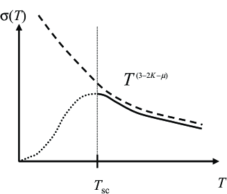
Figure 8: Schematic dependence of the temperature dependence of the conductivity. Above the MIT point $K>K_{c}$ the conductivity (dashed line) is power-law like with an exponent depending on the interactions. On the insulating side this behavior remains valid in the weak coupling regime, i. e. for temperatures above the crossover scale $T_{c}$ (see text).

When $H_{W}=0$ the conductance is simply $G=K$. Note that the fact that conductance is not $G=1$ for the pure system but depends on the interactions is in general an artefact, that has to be corrected depending on the systemsafi_pure_wire . However, since we focus here on the effect of a scattering potential, this is not important for our purpose.

A simple way to compute the conductance in (45) is again to iterate the RG flow until the cut-off is of the order of the size of the system. Up to that point the $q$ dependence can be neglected and $\sigma(\omega)\sim 1/M(\omega)$. The corrections to the conductance are thus given by :

$$\Delta G\propto\frac{1}{L}\frac{1}{M(l=\ln(L/\alpha))}\mbox{.}$$ (46)

Thus, with the scaling (39), one has :

$$\Delta G\propto L^{2K+\mu-4}\mbox{.}$$ (47)

For the disordered case, in the absence of any renormalization of the disorder, (47) leads to a variation of the resistance $\Delta R=1/\Delta G\propto L$ in the absence of interactions which is nothing but Ohm’s law. Interactions and renormalization of the parameter $K$ by disorder change this scaling giamarchi_loc ; giamarchi_moriond . Of course the renormalization of disorder also affects the exponents through the renormalization equations (13-14). The faster increase of the resistance with size is the sign of Anderson localization. As discussed before, the RG results can only be used if the renormalized scattering potential remains small compared to 1. This means that $\Delta G<e^{2}/h$. To go beyond, one needs to know the strong coupling fixed point. The lengthscale at which this happens is of course the Mott length for the commensurate potential and the localization length for the disorder as we now discuss in more details.

IV.2 Beyond the RG

In the metallic phase the RG gives the full physics of the system, up to arbitrarily low energy scales. On the insulating side, on the other hand, the RG flows to strong coupling. It thus defines a scale $l_{c}$ for which the function $\Xi$ becomes of order one. Below the lengthscale $L\sim\alpha e^{l_{c}}$ the RG still gives directly the physical properties, as shown for example on Fig 8. Note that this lengthscale can be quite large if the system is close to the MIT or for instance when the Fermi level is far from one of the main peaks. Beyond this lengthscale a knowledge of the strong coupling fixed point is in principle necessary to describe the physics of the system. Fortunately many of the properties can still be inferred directly from the Hamiltonian. Let us examine the various cases.

For the commensurate case, we know that the potential opens a gap in the spectrum. Thus, we can relate the crossover scale to the gap by :

$$\Delta/W\sim e^{-l_{c}}\sim\frac{\alpha}{\xi}\mbox{.}$$ (48)

Thus the RG gives directly the gap. The crossover scale is in this case the so-called Mott length $\xi$ above which the correlation functions have exponential decay. Similarly the conductivity decreases exponentially for temperatures below the gap.

In the disordered case, the situation is more subtle. The disorder does not open a gap, but we know that if it is strong enough, wavefunctions are exponentially localized, with a localization length of the order of the lattice spacing. One can thus again relate the crossover length to the localization length of the system by giamarchi_loc  :

$$\xi\propto\alpha e^{l_{c}}\mbox{.}$$ (49)

Because of the exponential localization of the wavefunctions, $\xi$ also defines a scale below which most of the interaction effects stop to be important.

Indeed the frequency dependence of the conductivity become for $\omega<\omega_{p}=u/\xi$, $\sigma(\omega)\sim\omega^{2}$ (up to log corrections) as for a non interacting system.

In the quasiperiodic case, the strong coupling fixed point is elusive so we can make only educated guesses. In the noninteracting case ($K=1$) for a point of the spectrum, the correlation functions decay as a power-law. It is thus unlikely that for the interacting case the strong coupling regime has a characteristic lengthscale in a similar way than the commensurate or disordered system. Thus the most likely possibility is that for the quasiperiodic case the length $\xi=\alpha e^{l_{c}}$ separates, two power-law regimes with different exponents. Since for the noninteracting quasiperiodic case, contrarily to the disordered case, the correlation functions are still power-law, interactions are likely to still play a role even in the strong coupling regime. One can thus naively expect in that case that the exponent in transport and other correlation functions still depend on the interaction strength, albeit probably in a different way than in the weak coupling regime. This crossover is schematically shown on Fig. 8.

The spectrum can also be inferred. For the non interacting case $K=1$ it consists in an infinite set of zero width bands. Clearly, the largest gaps must closed for $K=2$, as it is the case for the periodic system. Since there is, as shown in Section III.3.2, a MIT at $K=1$ for some filling fractions, the smallest gaps should close for $K=1+\epsilon$ ($\epsilon\ll 1$). We thus naturally expect larger and larger gaps to gradually close as the interactions become more and more attractive and the Luttinger parameter moves from $K=1$ to $K=2$. Such an evolution of the spectrum as a function of $K$ is depicted in Fig. 9. It would be interesting to check this scenario by numerical investigations.

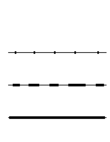
Figure 9: A possible evolution of the density of states as a function of the Luttinger liquid parameter $K$. For $K=1$ the spectrum is a set of measure zero and gaps are present almost everywhere. For $1<K<2$ the small gaps close as $K$ increases. For $K=2$ even the largest gaps are closed since even a periodic potential is irrelevant above $K=2$.

V Conclusion

We have studied in this paper a one-dimensional system of spinless fermions submitted to a quasiperiodic potential. Using a bosonization technique to treat the interactions exactly and the RG approach we had introduced in Ref. vidal_quasi_interactions_short, , we have investigated the effects of various types of quasiperiodic potentials known as precious potentials. We show that quasiperiodicity leads to a novel class of MIT as a function of the strength of the interactions, since for special filling factor the transition is pushed to the non interacting point (insulator for repulsive interactions and metallic for attractive ones). We have determined the critical exponents and the associated lengthscales and showed the universality of the results for all types of precious potentials. Our results are in good agreement with recent numerical investigations Hida_quasi_spinless_DMRG ; Hida_precious ; eilmes_mit_twoparticles .

We have also analyzed the transport properties such as the conductivity and the conductance. These quantities behave as power-laws with respect to the temperature (or with respect to the size for the conductance at $T=0$) with an interaction-dependent exponent. In the metallic regime, the RG flow converges towards a fixed point which allows to extract the full properties of the system. In the insulating regime, the system flows to a strong coupling regime at a lengthscale that we have determined. Above this lengthscale, it is necessary to analyze the physics with non pertubative method. Fortunately, one can still estimate qualitatively the behavior of some of the quantities. For instance, concerning the spectrum one expects, as the interaction becomes attractive (or equivalently as the Luttinger parameter reached $K>1$), that the smallest gaps start closing until $K=2$ where all gaps are closed. Similarly for the temperature dependence of the conductivity one expects below the crossover scale $T_{c}$, a power-law dependence of the conductivity. It would be interesting to check the above proposals in the numerical solutions, both for spinless Hida_quasi_spinless_DMRG and spinfull Hida_quasi_spinfull systems. More generally, the extension of these investigations to other types of potentials such as the Prouet-Thue-Morse or the paper-folding potentials Davis_paperfolding would be very useful since they also display a complex (dense) Fourier spectrum. Being able to tackle strong modulations would also allow for a comparison with potentials such as the Harper potentialseilmes_mit_twoparticles which at the perturbative level are similar to simple periodic ones.

Several other questions are prompted by our study. The first one concerns the temperature dependence of the conductivity. The formula we derived assume that there are phase breaking processes, so that the temperature acts indeed as a cut-off in the RG giamarchi_umklapp_1d . The validity of this assumption has been recently explicitly proven for the Mott (periodic) caserosch_conservation_1d . In that case, the phase breaking is provided by higher order periodicity (higher order umklapps). In the absence of such terms, the conductivity would remain infinite. It would be interesting to carry on the same type of memory matrix approximation for the quasiperiodic case. Second, it would be interesting to know if a correlated disorder could induce the same type of MIT as the one encountered here for the quasiperiodic system. Indeed, this type of disorder is susceptible to also produce a non trivial Fourier spectrum and thus to have a critical $K$ that depends explicitely on $k_{F}$.

To conclude, we address the question of experimental realizations to directly observe these effects. One could think about quasiperiodic chains in various devices. Since in one dimension there is a direct equivalence between spinless fermions and bosons haldane_bosons ; giamarchi_loc it is possible to investigate the physical properties of quasiperiodic chain in Josephson junction arrays fazio_josephson_junction_review . The advantage of such systems, besides the excellent control that one can have on the potential, is that we can reach the attractive regime. One could also realize a quasiperiodic chain using quantum dot arrays kouwenhoven_quantum_dots_1d or patterning of a quantum wire tarucha_quant_cond ; yacobi_quantumwire_conductance ; depicciotto_quantumwire_conductance . Finally, it would be interesting to check whether quasiperiodicity is relevant to describe systems such as DNA for which there has been recent transport measurementstran_dna_optics ; fink_dna_conductivity ; kazumov_dna_supra .

Appendix A Fourier Transform of Precious Mean Potentials

We consider a periodic one-dimensional chain decorated by a diagonal potential $W$ whose amplitudes on each site can take two discrete values $W_{A}=+\lambda/2$ or $W_{B}=-\lambda/2$ according to the substitution rule :

$$A\rightarrow A^{k}B,\hskip 8.61108ptB\rightarrow A\mbox{.}$$ (50)

To compute the Fourier transform of $W$, it is convenient to consider the $l^{th}$ order approximant of the potential obtained by iterating $(l-1)$ times the rule (50). We have represented below the first approximants of the Fibonacci sequence ($k$=1) :

$$\begin{array}[]{ll}l=1&B\\ l=2&A\\ l=3&AB\\ l=4&ABA\\ l=5&ABAAB\\ l=6&ABAABABA\mbox{.}\end{array}$$ (51)

For the $l^{th}$ order approximant, $W$ is thus a periodic potential with an elementary period $n_{l}=F_{l}$ containing $s_{l}=G_{l}$ elements $W_{A}$ and $p_{l}=G_{l-1}$ elements $W_{B}$ where $(F_{n})_{n\in{\bf N^{*}}}$ and $(G_{n})_{n\in{\bf N}}$ are the precious mean sequences defined by :

$$F_{1}=F_{2}=1\>;\>G_{0}=1,\>\>G_{1}=0$$ (52)

$$F_{n+1}=k\,F_{n}+F_{n-1}\>,\>\>\>\>\forall n>1$$ (53)

$$G_{n+1}=k\,G_{n}+G_{n-1}\>,\>\>\forall n>0\mbox{.}$$ (54)

In the quasiperiodic limit ($l\rightarrow\infty$), the ratio $s_{l}/p_{l}$ converges toward the Pisot solution $\tau={({k+\sqrt{k^{2}+4}})/2}$ of the equation $x^{2}=k\,x+1$. For $k=1,2,3,4$, $\tau$ is known as the golden, silver, bronze and chocolate mean respectively. Since $\tau$ is always irrationnal $(\forall k\in{\bf N^{*}})$, the length of the period becomes infinite, and the sequence is quasiperiodic.

The precious mean sequences can also be built by the Cut and Project algorithm starting from the usual ${\bf Z}^{2}$ lattice and choosing, for the cut slope, $\alpha_{l}=s_{l}/p_{l}$. In this case, one obtains a periodic structure with two types of lengths $L_{A}$ and $L_{B}$ distributed according to (50) but with a different origin than that given by (50). To establish a correspondence between the potential and the structure, one can, for example, affect $W_{A}$ (resp. $W_{B}$) to a site if the adjacent left segment of this site has length $L_{A}$ (resp. $L_{B}$) as displayed in Fig. 10.

Figure 10: A possible correspondence between the potential and the length applied to the $6^{th}$ approximant of the Fibonacci sequence ($n_{6}=8$, $s_{6}=5$, et $n^{\prime}_{6}=5$). The upper line gives the canonical numbering of the sites and the lower line, the conumbering.

For this type of tiling (codimension 1), it is possible to label each site according to their local environment and thus to classify them with respect to their on-site potentialmosseri_conumbering ; mosseri_conumbering_proceedings ; vidal_rauzy . This procedure, known as the conumbering scheme, allows to easily compute the Fourier transform of the potential, since it is simply expressed in terms of the so-called generating vector.

To achieve this conumering in our case, we introduce, following Ref.vidal_rauzy , the parallel space vector in the ${\bf Z}^{2}$ lattice for the $l^{th}$ order approximant ${\bf A}_{l}^{\parallel}=(G_{l},G_{l-1})$, and we look for the generating vector ${\bf g}_{l}$ determined by the condition $\det({\bf A}_{l}^{\parallel},{\bf g}_{l})=1$. Since, the precious mean sequences verify the relation :

$$G_{l}G_{l-2}-G_{l-1}^{2}=(-1)^{l}\mbox{,}$$ (55)

the generating vector is straightforwardly given by :

$${\bf g}_{l}=(-1)^{l}(G_{l-1},G_{l-2})\mbox{.}$$ (56)

After the projection step, each site can then be indexed by its conumber $j$ defined by $r_{j}=jn^{\prime}_{l}\>[n_{l}]$ for $j=[0,n-1]$ where $r_{j}$ denotes the canonical indexing (see Fig. 10), where $n^{\prime}_{l}=(-1)^{l}(G_{l-1}+G_{l-2})$ and where $n_{l}=G_{l}+G_{l-1}$. These two numbers ($n_{l}$ and $n^{\prime}_{l}$) are in fact the lengths of the vectors ${\bf A}_{l}^{\parallel}$ and ${\bf g}_{l}$ respectively measured in the ${\bf Z}^{2}$ lattice unit. Thus, all the sites whose conumber $j\in[0,s_{l}-1]$ (resp. $j\in[s_{l},n_{l}-1]$) have a potential $W_{A}$ (resp. $W_{B}$).

As a result, the Fourier transform of the potential is simply given by :

$$\hat{W}\left(q={2\pi m\over n}\right) = {1\over n}\sum_{j=0}^{n-1}W_{j}e^{iqr_{j}}$$ (57)

$$= {1\over n}\left(W_{A}\sum_{j=0}^{s-1}e^{iqjn^{\prime}[n]}+W_{B}\sum_{j=s}^{n-1}e^{iqjn^{\prime}[n]}\right)$$

$$= {\lambda\,e^{i{\pi mn^{\prime}(s-1)\over n}}\sin\left({\pi mn^{\prime}s\over n}\right)\over n\sin\left({\pi mn^{\prime}\over n}\right)}\mbox{,}$$

for integer values of $m\in[1,n-1]$ and :

$$\hat{W}(0)=\lambda(s-p)/2n\mbox{.}$$ (58)

Note that in (57), we have omitted the index $l$ for clarity.

Appendix B Bosonization of Spinless Fermions

Let us first consider free fermions, i. e. with $V=W=0$. The kinetic part of the Hamiltonian (1) is easily diagonalized via Fourier transform :

$$H_{t}=\sum_{k}\varepsilon(k)c^{\dagger}_{k}\,c_{k}\mbox{,}$$ (59)

where $c^{\dagger}_{k}=1/\sqrt{L}\>\sum_{j}e^{ikj}c^{\dagger}_{j}$ and $\varepsilon(k)=-2t\cos k$.

If one is interested in the low-energy properties of the system, the only relevant states are those standing around the Fermi points $\pm k_{F}$. One can thus linearize the dispersion relation around these points and obtain an effective Hamiltonian :

$$H_{t}=v_{F}\sum_{k}(k-k_{F})c^{\dagger}_{R,k}\,c_{R,k}-(k+k_{F})c^{\dagger}_{L,k}\,c_{L,k}\mbox{,}$$ (60)

where $v_{F}=2t\sin k_{F}$ is the Fermi velocity and where we have introduced the right $R$ (respectively the left $L$) movers fermions with momentum close to $+k_{F}$ (respectively to $-k_{F}$).

We now introduce the fermions fields :

$$\psi_{\nu}(x) = {1\over\sqrt{L}}\sum_{k}e^{ikx}c_{\nu,k}\mbox{,}$$ (61)

where $\nu=R$ or $L$, so that the Hamiltonian (60) writes in the continuum limit :

$$H_{t}=-iv_{F}\int dx\ \psi^{\dagger}_{R}(x)\partial_{x}\psi_{R}(x)-\psi^{\dagger}_{L}(x)\partial_{x}\psi_{L}(x)\mbox{.}$$ (62)

We also introduce the right and left Fourier components of the fermions density operators :

$$\rho_{\nu}(q) = \sum_{k}c^{\dagger}_{\nu,k+q}c_{\nu,k}\mbox{,}$$ (63)

which satisfy bosonic commutation relations :

$$\left[\rho_{R}(-q),\rho_{R}(q^{\prime})\right] = {qL\over 2\pi}\delta_{qq^{\prime}}\mbox{,}$$ (64)

$$\left[\rho_{L}(-q),\rho_{L}(q^{\prime})\right] = -{qL\over 2\pi}\delta_{qq^{\prime}}\mbox{,}$$ (65)

$$\left[\rho_{R}(q),\rho_{L}(q^{\prime})\right] = 0\mbox{.}$$ (66)

The commutation relations of these operators with the Hamiltonian $H_{t}$ :

$$\left[H_{t},\rho_{R}(q)\right] = v_{F}\>q\>\rho_{R}(q)\mbox{,}$$ (67)

$$\left[H_{t},\rho_{L}(q)\right] = -v_{F}\>q\>\rho_{L}(q)\mbox{,}$$ (68)

explicitely show that $\rho_{\nu}(q)$ generate eigenstates of $H_{t}$ with the energy $v_{F}q$. This allows to write the kinetic energy as a bilinear operator in the bosonic fields :

$$H_{t}={\pi v_{F}\over L}\sum_{q\neq 0}\left[\rho_{R}(q)\rho_{R}(-q)+\rho_{L}(q)\rho_{L}(-q)\right]\mbox{,}$$ (69)

or in the real space :

$$H_{t}=\pi v_{F}\int dx\left[\rho_{R}(x)^{2}+\rho_{L}(x)^{2}\right]\mbox{,}$$ (70)

where $\rho_{\nu}(x)=\psi^{\dagger}_{\nu}(x)\psi_{\nu}(x)$ for $\nu=R$ or $L$.

We now introduce the fields $\phi$ and $\theta$ :

$$\phi(x) = {-i\pi\over L}\sum_{q\neq 0}{(\rho_{R}(q)+\rho_{L}(q))\over q}e^{-iqx}\mbox{,}$$ (71)

$$\theta(x) = {i\pi\over L}\sum_{q\neq 0}{(\rho_{R}(q)-\rho_{L}(q))\over q}e^{-iqx}\mbox{,}$$ (72)

together with their conjugate momenta :

$$\Pi_{\phi}(x) = \displaystyle{{1\over\pi}}\partial_{x}\theta(x)\mbox{,}$$ (73)

$$= \displaystyle{{1\over L}}\sum_{q\neq 0}\left(\rho_{R}(q)-\rho_{L}(q)\right)e^{-iqx}\mbox{,}$$ (74)

$$= \rho_{R}(x)-\rho_{L}(x)\mbox{,}$$ (75)

$$\Pi_{\theta}(x) = \displaystyle{{1\over\pi}}\partial_{x}\phi(x)\mbox{,}$$ (76)

$$= \displaystyle{{-1\over L}}\sum_{q\neq 0}\left(\rho_{R}(q)+\rho_{L}(q)\right)e^{-iqx}\mbox{,}$$ (77)

$$= -\rho_{R}(x)-\rho_{L}(x)\mbox{,}$$ (78)

which obey the canonical commutation rules :

$$\left[\phi(x),\Pi_{\phi}(x)\right] = i\delta(x-x^{\prime})\mbox{,}$$ (79)

$$\left[\theta(x),\Pi_{\theta}(x)\right] = i\delta(x-x^{\prime})\mbox{.}$$ (80)

This finally allows to rewrite the kinetic energy :

$$H_{t}={v_{F}\over 2\pi}\int dx\left[(\pi\Pi)^{2}+(\partial_{x}\phi)^{2}\right]\mbox{,}$$ (81)

with $\Pi=\Pi_{\phi}$, which is the Hamiltonian of a one-dimensional elastic string. The fermions operators, and thus, all physical quantites (charge density wave, Cooper pairs density,…), can be easily expressed in terms of the $\phi$ and $\Pi$ fields. The correspondence between the two sets of operators are given by the following relations :

$$\psi_{R}^{\dagger}(x) = {1\over\sqrt{2\pi\alpha}}U^{\dagger}_{R}e^{i(\phi(x)-\theta(x))}$$ (82)

$$\psi_{L}^{\dagger}(x) = {1\over\sqrt{2\pi\alpha}}U^{\dagger}_{L}e^{-i(\phi(x)+\theta(x))}\mbox{,}$$ (83)

$\alpha$ being an ultraviolet cut-off and $\theta(x)$ being defined by : $\theta(x)=\pi\int_{-\infty}^{x}\ \Pi(x^{\prime})dx^{\prime}$. The operators $U_{R}$ and $U_{L}$ are anticommuting operators which ensure the correct commutation relations of the fermions operators. Note that these operators give essentially vanishing contributions in the thermodynamical limit and can be safely ignored, at least in the case of single chain systems.

The great advantage of this bosonic formulation is that the interaction term $H_{V}$ can be almost trivially taken into account. Let us consider, for instance, a two-body interaction :

$$H_{V}={1\over 2}\int dx\int dx^{\prime}\rho(x)\ V(x-x^{\prime})\>\rho(x^{\prime})\mbox{,}$$ (84)

where $\rho(x)$ is the fermion density operator on site $x$.

If one is only interested in the low-energy physics, the fermion field operator $\psi(x)$ writes :

$$\psi(x)=e^{ik_{F}x}\psi_{R}(x)+e^{-ik_{F}x}\psi_{L}(x)\mbox{,}$$ (85)

which correctly describes the low-energy behavior of the particle-hole and particle-particle density state. It follows that the density operator expresses as :

$$\rho(x) = \psi^{\dagger}(x)\psi(x)\mbox{,}$$ (86)

$$= \psi^{\dagger}_{R}(x)\psi_{R}(x)+\psi^{\dagger}_{L}(x)\psi_{L}(x)+e^{-2ik_{F}x}\psi^{\dagger}_{R}(x)\psi_{L}(x)+e^{2ik_{F}x}\psi^{\dagger}_{L}(x)\psi_{R}(x)\mbox{,}$$ (87)

$$= \rho_{R}(x)+\rho_{L}(x)+e^{-2ik_{F}x}\psi^{\dagger}_{R}(x)\psi_{L}(x)+e^{2ik_{F}x}\psi^{\dagger}_{L}(x)\psi_{R}(x)\mbox{,}$$ (88)

$$= -{1\over\pi}\partial_{x}\phi(x)+{1\over\pi\alpha}\cos(2\phi(x)-2k_{F}x)\mbox{,}$$ (89)

and :

$$\rho(x)\rho(x^{\prime}) = \rho_{R}(x)\rho_{R}(x^{\prime})+\rho_{L}(x)\rho_{L}(x^{\prime})+\rho_{R}(x)\rho_{L}(x^{\prime})+\rho_{L}(x)\rho_{R}(x^{\prime})+$$

$$e^{-i2k_{F}(x-x^{\prime})}\>\psi^{\dagger}_{R}(x)\psi_{L}(x)\psi^{\dagger}_{L}(x^{\prime})\psi_{R}(x^{\prime})+$$

$$e^{i2k_{F}(x-x^{\prime})}\>\psi^{\dagger}_{L}(x)\psi_{R}(x)\psi^{\dagger}_{R}(x^{\prime})\psi_{L}(x^{\prime})+$$

oscillating terms.

In the case of short-range interactions the remaining oscillating terms are supposed to give negligible contributions and we keep only terms behaving like $e^{-i2k_{F}(x-x^{\prime})}$.

If one consider local interactions, one can write the interaction term in the general form :

$$H_{V}=\int dx\> {g_{4}\over 2}\bigg{[}\rho_{R}(x)\rho_{R}(x)+\rho_{L}(x)\rho_{L}(x)\bigg{]}+$$ (91)

$$g_{2}\>\rho_{R}(x)\rho_{L}(x)\mbox{,}$$

with the standard notations of $g-ology$. Gathering (81) and (91) and the Hamiltonian $H_{0}(t,V)$ then becomes :

$$H_{0}(t,V)={1\over 2\pi}\int dx\>(uK)(\pi\Pi)^{2}+\left({u\over K}\right)(\partial_{x}\phi)^{2}\mbox{,}$$ (92)

where we have introduced the parameters $u$ and $K$ (Luttinger parameter) given by :

$$u = \sqrt{\left(v_{F}+{g_{4}\over 2\pi}\right)^{2}-\left({g_{2}\over 2\pi}\right)^{2}}\mbox{,}$$ (93)

$$K = \sqrt{{2\pi v_{F}+g_{4}-g_{2}\over 2\pi v_{F}+g_{4}+g_{2}}}\mbox{.}$$ (94)

The Hamiltonian (92) can still be interpreted as the Hamiltonian of an elastic string with effective parameters $u$ and $K$.

For the model considered here, the interaction term writes :

$$V\sum_{i}n_{i}n_{i+1}\>\rightarrow\lim_{a\rightarrow 0}Va\int dx\>\rho(x)\,\rho(x+a)\mbox{.}$$ (95)

This expression can also be written as (91) for $V\ll t$ with : $g_{4}=g_{2}=2V(1-\cos(2k_{F}a))$. Note that, in the non interacting case one has $K=1$ and $u=v_{F}=2t\sin(k_{F}a)$. For repulsive interactions ($V>0$), $K<1$ while the attractive case ($V<0$) leads to $K>1$. A remarkable fact is that the representation (92) is, in fact, completely generalhaldane_xxzchain ; haldane_bosonisation and gives the correct low-energy description of the system, even when the interactions are strong provided the correct $u$ and $K$ parameters are used.

For example for $k_{F}=\pi/2$ one has for the interaction (95) :

$$\frac{V}{2t} = -\cos\left({\pi\over 2K}\right)$$ (96)

$$u = \frac{2Kt}{2K-1}\sin\left(\pi\left(1-\frac{1}{2K}\right)\right)\mbox{.}$$ (97)

Concerning the bosonization of $H_{W}$, one straightforwardly obtains, in the continuum limit :

$$H_{W}=\int dx\>W(x)\,\rho(x)=\int dx\>W(x)\,\left(-{1\over\pi}\partial_{x}\phi(x)+{1\over\pi\alpha}\cos(2\phi(x)-2k_{F}x)\right)\mbox{.}$$ (98)

Appendix C Renormalization Group Equations

The aim of this appendix is to derive the RG equations used in Section II, following the method of Ref. giamarchi_spin_flop, .
We evaluate the correlation function $R(x,\tau,x^{\prime},\tau^{\prime})$ perturbatively at second order in power of the coupling constant $g$ :

$$\left\langle T_{\tau}e^{i\sqrt{2}\phi(x^{\prime},\tau^{\prime})}e^{-i\sqrt{2}\phi(x,\tau)}\right\rangle = I_{0}-{g\over u(2\pi\alpha)^{2}}\>I_{1}+{1\over 2}{g^{2}\over u^{2}(2\pi\alpha)^{4}}\>I_{2}+o(g^{3})\ \mbox{,}$$ (99)

with :

$$I_{0} = \left\langle T_{\tau}e^{i\sqrt{2}\phi(x^{\prime},\tau^{\prime})}e^{-i\sqrt{2}\phi(x,\tau)}\right\rangle_{0}$$ (100)

$$I_{1} = \sum_{Q}{\hat{W}(Q)}\int d^{2}{\bf r}_{1}\left\langle T_{\tau}e^{i\sqrt{2}\phi(x^{\prime},\tau^{\prime})}e^{-i\sqrt{2}\phi(x,\tau)}\left[e^{i\left[2\phi(x_{1},\tau_{1})+Q^{-}x_{1}\right]}+e^{i\left[-2\phi(x_{1},\tau_{1})+Q^{+}x_{1}\right]}\right]\right\rangle_{0}\mbox{,}$$ (101)

with $Q^{\pm}=Q\pm 2k_{F}$ and :

$$I_{2} = \sum_{Q_{1},\,Q_{2}}{\hat{W}(Q_{1})}{\hat{W}(Q_{2})}\int d^{2}{\bf r}_{1}\int d^{2}{\bf r}_{2}\left\langle T_{\tau}e^{i\sqrt{2}\phi(x^{\prime},\tau^{\prime})}e^{-i\sqrt{2}\phi(x,\tau)}\right.\times$$

$$\left[e^{i\left[2\phi(x_{1},\tau_{1})+Q^{-}_{1}x_{1}\right]}+e^{i\left[-2\phi(x_{1},\tau_{1})+Q^{+}_{1}x_{1}\right]}\right]\left.\left[e^{i\left[2\phi(x_{2},\tau_{2})+Q^{-}_{2}x_{2}\right]}+e^{i\left[-2\phi(x_{2},\tau_{2})+Q^{+}_{2}x_{2}\right]}\right]\right\rangle_{0}^{c}\mbox{,}$$

where $\langle\rangle_{0}$ denotes the average performed with respect to the free action, i. e. with $g=0$. The index $c$ in Eq.(C) refers to the connected correlation function with respect to the quantities indexed by 1 and 2.

The average in Eqs. (100) (101) and (C) are easily performed using the relation :

$$\left\langle T_{\tau}e^{ic_{1}\phi(x_{1},\tau_{1})}e^{ic_{2}\phi(x_{2},\tau_{2})}\dots e^{ic_{n}\phi(x_{n},\tau_{n})}\right\rangle_{0}\simeq e^{{K\over 2}\sum_{i>j}c_{i}c_{j}\ln{|{\bf r}_{i}-{\bf r}_{j}|\over\alpha}}\mbox{,}$$ (103)

when $|{\bf r}_{i}-{\bf r}_{j}|\gg\alpha$. Note also that the expression (103) vanishes if the “neutrality” condition, $\sum_{i}c_{i}=0$, is not satisfied. One thus has :

$$I_{0} = \left\langle T_{\tau}e^{i\sqrt{2}\phi(x^{\prime},\tau^{\prime})}e^{-i\sqrt{2}\phi(x,\tau)}\right\rangle_{0}$$ (104)

$$= e^{i{\sqrt{2}K\over u}\int_{x^{\prime}}^{x}W(y)dy}\left\langle T_{\tau}e^{i\sqrt{2}\tilde{\phi}(x^{\prime},\tau^{\prime})}e^{-i\sqrt{2}\tilde{\phi}(x,\tau)}\right\rangle_{0}$$ (105)

$$= e^{i{\sqrt{2}K\over u}\int_{x^{\prime}}^{x}W(y)dy}\>e^{-F({\bf r-r^{\prime}})}\mbox{,}$$ (106)

with $F({\bf r-r^{\prime}})=K\ln|{\bf r-r^{\prime}}|/\alpha$.

Note that $I_{1}$ vanishes since it does not respect the neutrality condition. It follows that the first non trivial contribution of the potential is provided by the term $I_{2}$. Keeping in (C) the terms satisfying the neutrality condition and performing the average over the fields one obtains :

$$I_{2} = e^{i{\sqrt{2}K\over u}\int_{x^{\prime}}^{x}W(y)dy}\>e^{-F({\bf r-r^{\prime}})}\times$$

$$\sum_{Q_{1},\,Q_{2}}{\hat{W}(Q_{1})}{\hat{W}(Q_{2})}\int d^{2}{\bf r}_{1}\int d^{2}{\bf r}_{2}\>e^{-2\,F({\bf r}_{1}-{\bf r}_{2})}e^{i{2K\over u}\int_{x_{2}}^{x_{1}}W(y)dy}\times$$

$$\bigg{[}e^{-\sqrt{2}\,F({\bf r}-{\bf r}_{1})+\sqrt{2}\,F({\bf r}-{\bf r}_{2})+\sqrt{2}\,F({\bf r^{\prime}}-{\bf r}_{1})-\sqrt{2}\,F({\bf r^{\prime}}-{\bf r}_{2})}-1\bigg{]}\bigg{[}e^{i\left(Q^{-}_{1}x_{1}+Q^{+}_{2}x_{2}\right)}+e^{i\left(Q^{+}_{1}x_{2}+Q^{-}_{2}x_{1}\right)}\bigg{]}\mbox{.}$$

At this order the potential enters only through a pure phase and does not drastically affects the long distance behavior. Anyway, a choice of a vanishing average value for the potential renders this effect negligible.

The integration over ${\bf r}_{1}$ et ${\bf r}_{2}$ is performed with the following variable changes :

$${\bf r}_{1}={\bf R}+{\delta{\bf r}\over 2}\>,\>\>{\bf r}_{2}={\bf R}-{\delta{\bf r}\over 2}\mbox{,}$$ (108)

since, due to the factor $\>e^{-2\,F({\bf r}_{1}-{\bf r}_{2})}$ in Eq.(C) the non vanishing contributions are given by “points” separated by small values of $\delta{\bf r}={\bf r}_{1}-{\bf r}_{2}$. If the potential is translation invariant, the term $e^{i{2K\over u}\int_{x_{2}}^{x_{1}}W(y)dy}$ does only depends on $x_{1}-x_{2}$ and is thus of order one for small $\delta{\bf r}$. Of course, in the quasiperiodic case, this is no longer true. Nevertheless, if one is only interested by the intrinsic properties of the potential, it is reasonable to perform an average over all the possible choice of the sequence origin. Then, we can also consider that $e^{i{2K\over u}\int_{x_{2}}^{x_{1}}W(y)dy}$ only depends on $x_{1}-x_{2}$ and replace it by 1.

At leading order in $\delta{\bf r}$, one has :

$$F({\bf r}-{\bf r}_{1})-F({\bf r}-{\bf r}_{2})-F({\bf r^{\prime}}-{\bf r}_{1})+F({\bf r^{\prime}}-{\bf r}_{2})=\delta{\bf r}.\nabla_{\bf R}\left[F({\bf r}^{\prime}-{\bf R})-F({\bf r}-{\bf R})\right]+o(\delta{\bf r})^{3}\mbox{.}$$ (109)

On the other hand, with ${\bf R}=(X,Y)$ et $\delta{\bf r}=(\delta x,\delta y)$ one has :

$$Q^{-}_{1}x_{1}+Q^{+}_{2}x_{2}=\left(Q_{1}+Q_{2}\right)X+\left(Q^{-}_{1}-Q^{+}_{2}\right){\delta x\over 2}\mbox{,}$$ (110)

and :

$$Q^{+}_{1}x_{2}+Q^{-}_{2}x_{1}=\left(Q_{1}+Q_{2}\right)X+\left(Q^{-}_{2}-Q^{+}_{1}\right){\delta x\over 2}\mbox{,}$$ (111)

which implies that the integration over the variable $X$ selects the contributions $Q_{1}=-Q_{2}=Q$ in the sum over $Q_{1}$ and $Q_{2}$. Also, taking the fact that the potential $W$ can be taken as real one has $\hat{W}(Q)=\hat{W}^{*}(-Q)$ and :

$$I_{2} = e^{i{\sqrt{2}K\over u}\int_{x^{\prime}}^{x}W(y)dy}\>e^{-F({\bf r-r^{\prime}})}\>\sum_{Q}\left|\hat{W}(Q)\right|^{2}\int d^{2}{\bf R}\int d^{2}\delta{\bf r}\>\>e^{-2\,F(\delta{\bf r})}\bigg{[}e^{i\left(Q^{-}\delta x\right)}+e^{-i\left(Q^{+}\delta x\right)}\bigg{]}\times$$

$$\bigg{(}\delta{\bf r}.\nabla_{\bf R}\left[F({\bf r}^{\prime}-{\bf R})-F({\bf r}-{\bf R})\right]\bigg{)}^{2}\mbox{.}$$

Let us now define : $\zeta=F({\bf r}^{\prime}-{\bf R})-F({\bf r}-{\bf R})$. One has :

$$(\delta{\bf r}.\nabla_{\bf R}\>\zeta)^{2}=(\delta x\>\partial_{X}\>\zeta)^{2}+(\delta y\>\partial_{Y}\>\zeta)^{2}+2\delta x\>\delta y\>\partial_{X}\>\zeta\>\partial_{Y}\>\zeta\mbox{.}$$ (113)

By parity only the two first terms would survive to the integral over $\delta y$ (or $\delta x$). On the other hand, the integral over $\bf R$ is easily performed and leads to two kind of terms :

$$\int d^{2}{\bf R}\>\zeta\left(\partial^{2}_{X}+\partial^{2}_{Y}\right)\zeta=-4\pi K^{2}\ln{|{\bf r-r^{\prime}}|\over\alpha}\mbox{,}$$ (114)

and :

$$\int d{\bf R}\>\zeta\left(\partial^{2}_{X}-\partial^{2}_{Y}\right)\zeta=-2\pi\cos 2\theta_{\bf r-r^{\prime}}\mbox{,}$$ (115)

where $\theta_{\bf r-r^{\prime}}$ is the angle between the vector $(x,\tau)$ and the $x$ axis. The occurence of the second term comes from the fact that the free correlation function $F$ writes, in fact, as :

$$F({\bf r-r^{\prime}})=K\ln{|{\bf r-r^{\prime}}|\over\alpha}+d\cos(2\theta_{\bf r-r^{\prime}})\mbox{,}$$ (116)

where $d$ parametrizes the anisotropy between the space and time direction. One has $d=0$ in the original Hamiltonian but, as seen in Eq.(115), this anisotropy is generated by renormalization. Ultimately, this is equivalent to a renormalizaton of the Fermi velocity $u$. However, since the anisotropy itself is of order $g^{2}$, the correction to $u$ can be neglected in this calculation.

Gathering the preceeding results one thus finds :

$$I_{2} = e^{i{\sqrt{2}K\over u}\int_{x^{\prime}}^{x}W(y)dy}\>e^{-F({\bf r-r^{\prime}})}\>2\pi K^{2}\>\sum_{Q}\left|\hat{W}(Q)\right|^{2}\ln{|{\bf r}-{\bf r}^{\prime}|\over\alpha}\times$$

$$\int d\delta{\bf r}\>\delta^{2}{\bf r}\>e^{-2\,F(\delta{\bf r})}\bigg{[}e^{i\left(Q^{-}\delta x\right)}+e^{-i\left(Q^{+}\delta x\right)}\bigg{]}\mbox{,}$$

which also reads :

$$I_{2} = e^{i{\sqrt{2}K\over u}\int_{x^{\prime}}^{x}W(y)dy}\>e^{-F({\bf r-r^{\prime}})}\>2\pi K^{2}\>\sum_{Q}\left|\hat{W}(Q)\right|^{2}\ln{|{\bf r}-{\bf r}^{\prime}|\over\alpha}\times$$

$$2\pi\alpha^{3}\int_{\alpha}^{+\infty}d\delta r\>\left({\delta r\over\alpha}\right)^{3-2K}\bigg{[}\mbox{J}_{0}(Q^{+}\delta r)+\mbox{J}_{0}(Q^{-}\delta r)\bigg{]}\mbox{,}$$

where $\mbox{J}_{0}$ is a Bessel function.

Finally the correlation function $R(x,\tau,x^{\prime},\tau^{\prime})$ writes :

$$\left\langle T_{\tau}e^{i\sqrt{2}\phi(x^{\prime},\tau^{\prime})}e^{-i\sqrt{2}\phi(x,\tau)}\right\rangle_{g} = e^{i{\sqrt{2}K\over u}\int_{x^{\prime}}^{x}W(y)dy}\>e^{-F({\bf r-r^{\prime}})}\left\{1+{g^{2}K^{2}\over 8\pi^{2}u^{2}}\ln{|{\bf r}-{\bf r}^{\prime}|\over\alpha}\sum_{Q}\left|\hat{W}(Q)\right|^{2}\right.\times$$

$$\left.\int_{\alpha}^{+\infty}{d\delta r\over\alpha}\>\left({\delta r\over\alpha}\right)^{3-2K}\bigg{[}\mbox{J}_{0}(Q^{-}\delta r)+\mbox{J}_{0}(Q^{+}\delta r)\bigg{]}\right\}\mbox{.}$$

By re-exponentiation one has :

$$R(x,\tau,x^{\prime},\tau^{\prime})=\left({\alpha\over|{\bf r-r^{\prime}}|}\right)^{K_{eff}}\mbox{,}$$ (120)

with :

$$K_{eff}=K-{K^{2}\over 2}\sum_{Q}y_{Q}^{2}\int_{\alpha}^{+\infty}{d\delta r\over\alpha}\>\left({\delta r\over\alpha}\right)^{3-2K}\bigg{[}\mbox{J}_{0}(Q^{+}\delta r)+\mbox{J}_{0}(Q^{-}\delta r)\bigg{]}\mbox{,}$$ (121)

with $y_{Q}=\lambda\alpha\hat{W}(Q)/u$.

To derive the RG equation, one has to consider an infinitesimal variation of the running cut-off $\alpha(l)$ to $\alpha(l)e^{dl}$ in Eq.(121). This leads to :

$${dK\over dl} = -K^{2}\,\Xi(l)$$ (122)

$${dy_{Q}\over dl} = (2-K)\,y_{Q}\mbox{,}$$ (123)

with :

$$\Xi(l)={1\over 2}\sum_{Q}y_{Q}^{2}\left[\mbox{J}_{0}(Q^{+}\alpha(l))+\mbox{J}_{0}(Q^{-}\alpha(l))\right]\mbox{.}$$ (124)

Here one has to note that the use of a sharp cut-off in real space leads to the occurrence of Bessel function ${\mbox{J}}_{0}$ . This choice is in fact not satisfying since it does not ensure the convergence of the sum (124). This is the reason why we have considered more general cut-off procedures for which ${\mbox{J}}_{0}$ is replaced by faster decreasing functions which typically satisfy (16-17).

Appendix D Memory function

In a normal metal (finite conductivity at $\omega=0$) the Kubo formula :

$$\sigma(\omega)=\frac{i}{\omega}\left[\frac{2uK}{\pi}+\chi(\omega)\right]\mbox{,}$$ (125)

implies that $\chi(0)=-2uK/\pi$. Then (125) can be reexpressed in terms of a meromorphic function $M$ through :

$$\sigma(\omega)=\frac{i2uK}{\pi}\frac{1}{\omega+M(\omega)}\mbox{,}$$ (126)

where $M$ is given by :

$$M(\omega)=\frac{\omega\chi(\omega)}{\chi(0)-\chi(\omega)}\mbox{.}$$ (127)

The interest of the function $M$ lies in the fact that, contrarily to the conductivity itself, one can expect $M$ to have a well behaved expansion in the scattering potential $H_{W}$. Indeed in a simple hydrodynamic approximation $M(\omega\to 0)$ would simply be the inverse relaxation time $M\sim i/\tau$, leading to the standard Lorentzian broadening of the Drude peak. Another way to formulate it is that a perturbative calculation of the memory function is close to a perturbative calculation of the resistivity. In the lowest order in the scattering potential $H_{W}$ one gets :

$$\chi(0)-\chi(\omega)\sim\chi(0)\mbox{,}$$ (128)

and :

$$\omega\chi(\omega)=[\langle F;F\rangle_{\omega}^{0}-\langle F;F\rangle^{0}_{\omega=0}]/\omega\mbox{,}$$ (129)

where $F$ operator takes into account the fact that the current is not a conserved quantity $F=[j,H]$ and $\langle F;F\rangle_{\omega}^{0}$ stands for the retarded correlation function of the operator $F$ at frequency $\omega$. Since $F$ is itself proportional to the scattering potential, at lowest order the average can be computed with the Hamiltonian in the absence of scattering potential. This leads to :

$$M(\omega)=\frac{[\langle F;F\rangle_{\omega}^{0}-\langle F;F\rangle^{0}_{\omega=0}]/\omega}{-\chi(0)}\mbox{,}$$ (130)

where $\langle\rangle^{0}$ stands for an average with (3) only. Since all averages are to be computed with the quadratic Hamiltonian (3) only, the computation of $M$ is now feasible.

References

- (1) D. Shechtman, I. Blech, D. Gratias, and J. W. Cahn, Phys. Rev. Lett. 53, 1951 (1984).
- (2) C. Sire, in Lectures on Quasicrystals, edited by F. Hippert and D. Gratias (Editions de Physique, Les Ulis France, 1994), p. 505.
- (3) H. Schulz-Baldes and J. Bellissard, J. Stat. Phys. 91, 991 (1998).
- (4) F. Piéchon, Phys. Rev. Lett. 76, 4375 (1996).
- (5) C. Sire and R. Mosseri, J. Phys. (Paris) 50, 3447 (1989).
- (6) R. Ketzmerick, G. Petschel, and T. Geisel, Phys. Rev. Lett. 69, 695 (1992).
- (7) S. Roche, D. Mayou, and G. Trambly de Laissardiere, J. Math. Phys. 38, 1794 (1997).
- (8) H. Hiramoto, J. Phys. Soc. Jpn. 59, 811 (1990).
- (9) J. C. Chaves and I. I. Satija, Phys. Rev. B 55, 14076 (1997).
- (10) J. C. Chaves, I. I. Satija, and M. M. Doria, cond-mat/9803103.
- (11) A. Eilmes, R. A. Römer, C. Schuster, and M. Schreiber (2001), cond-mat/0102251.
- (12) J. Vidal, D. Mouhanna, and T. Giamarchi, Phys. Rev. Lett. 83, 3908 (1999).
- (13) T. Giamarchi, Phys. Rev. B 44, 2905 (1991).
- (14) T. Giamarchi, Physica B 230-232, 975 (1997).
- (15) W. Apel, J. Phys. C 15, 1973 (1982).
- (16) T. Giamarchi and H. J. Schulz, Phys. Rev. B 37, 325 (1988).
- (17) J. Sólyom, Adv. Phys. 28, 209 (1979).
- (18) V. J. Emery, Highly Conducting One-Dimensional Solids (Plenum Press, New York and London, 1979), p. 247.
- (19) H. J. Schulz, in Mesoscopic quantum physics, Les Houches LXI, edited by E. Akkermans, G. Montambaux, J. L. Pichard, and J. Zinn-Justin (Elsevier, Amsterdam, 1995), p. 533.
- (20) J. Voit, Rep. Prog. Phys. 58, 977 (1995).
- (21) E. Kolomeisky, Phys. Rev. B 47, 6193 (1993).
- (22) D. Sen and S. Lal, Europhys. Lett. 52, 337 (2000).
- (23) D. Sen and S. Lal, Phys. Rev. B 61, 9001 (2000).
- (24) J. Vidal, D. Mouhanna, and T. Giamarchi (2000), “Interactions in quasicrystals”, in Proceedings of Xth MBX conference, to be published by World Scientific (ed. R. Bishop, K. Gernoth, N. Walet and Yang Xian), cond-mat/9912343.
- (25) K. Hida, J. Phys. Soc. Jpn. 68, 3177 (1999).
- (26) K. Hida, J. Phys. Soc. Jpn. 69, 311 (2000).
- (27) V. Mastropietro (1998), cond-mat/9810128.
- (28) K. Hida, Phys. Rev. Lett. 86, 1331 (2001).
- (29) F. D. M. Haldane, Phys. Rev. Lett. 45, 1358 (1980).
- (30) F. D. M. Haldane, J. Phys. C 14, 2585 (1981).
- (31) V. L. Berezinskii, Zh. Eksp. Teor. Fiz. 59, 907 (1970).
- (32) V. L. Berezinskii, Sov. Phys. JETP 32, 493 (1971).
- (33) J. M. Kosterlitz and D. J. Thouless, J. Phys. C 6, 1181 (1973).
- (34) J. Peyrière, in Beyond Quasicrystals, edited by F. Axel and D. Gratias (Les Editions de Physique, Les Ulis, 1995), p. 465.
- (35) T. Giamarchi, Phys. Rev. B 46, 342 (1992).
- (36) W. Götze and P. Wölfle, Phys. Rev. B 6, 1226 (1972).
- (37) M. Ogata and H. Fukuyama, Phys. Rev. Lett. 73, 468 (1994).
- (38) T. Giamarchi and H. Maurey, in Correlated fermions and transport in mesoscopic systems, edited by T. Martin, G. Montambaux, and J. Tran Thanh Van (Editions Frontières, Gif sur Yvette, France, 1996), cond-mat/9608006.
- (39) I. Safi and H. J. Schulz, Phys. Rev. B 52, R17040 (1995).
- (40) C. Davis and D. E. Knuth, Recr. Math. 3, 133 (1970).
- (41) A. Rosch and N. Andrei, Phys. Rev. Lett. 85, 1092 (2000).
- (42) F. D. M. Haldane, Phys. Rev. Lett. 47, 1840 (1981).
- (43) R. Fazio and H. van der Zant (2000), cond-mat/0011152.
- (44) L. P. Kouwenhoven and et al., Phys. Rev. Lett. 65, 361 (1990).
- (45) S. Tarucha, T. Honda, and T. Saku, Sol. State Comm. 94, 413 (1995).
- (46) A. Yacobi and et al., Phys. Rev. Lett. 77, 4612 (1996).
- (47) R. de Picciotto and et al., Nature 411, 51 (2001).
-
(48)
P. Tran,
B. Alavi, and
G. Gruner,
Phys. Rev. Lett. 85,
1564 (2000).
- (49) H. W. Fink and C. Schonenberger, Nature 398, 407 (2001).
- (50) A. Y. Kazumov and et al., Science 291, 280 (2001).
- (51) R. Mosseri, in Proceedings of the 3rd International Meeting on Quasicrystals, edited by J. Y. et al. (World Scientific, Singapore, 1990), p. 129.
- (52) R. Mosseri, in Proceedings in Physics Vol. 32, Universalities in Condensed Matter, edited by R. J. et al. (Springer-Verlag, Berlin Heidelberg, 1988), p. 9.
- (53) J. Vidal and R. Mosseri, J. Phys. A 34, 3927 (2001).
- (54) T. Giamarchi and H. J. Schulz, J. Phys. (Paris) 49, 819 (1988).