(submitted to Phys. Rev. B)
Composition, structure and stability of RuO₂(110)
as a function of oxygen pressure

Abstract

Using density-functional theory (DFT) we calculate the Gibbs free energy to determine the lowest-energy structure of a RuO₂(110) surface in thermodynamic equilibrium with an oxygen-rich environment. The traditionally assumed stoichiometric termination is only found to be favorable at low oxygen chemical potentials, i.e. low pressures and/or high temperatures. At realistic O pressure, the surface is predicted to contain additional terminal O atoms. Although this O excess defines a so-called polar surface, we show that the prevalent ionic model, that dismisses such terminations on electrostatic grounds, is of little validity for RuO₂(110). Together with analogous results obtained previously at the (0001) surface of corundum-structured oxides, these findings on (110) rutile indicate that the stability of non-stoichiometric terminations is a more general phenomenon on transition metal oxide surfaces.

]

I Introduction

Density-functional theory (DFT) is often argued to be a zero temperature, zero pressure technique. As such, the results of static total energy calculations at surfaces have to be transferred with considerable care to typical high-pressure applications like e.g. catalysis — a situation which finds its correspondence in the experiment in form of the ex-situ methods of ultra high vacuum (UHV) surface science. Unfortunately, often enough an extrapolation of the low-pressure results to technical processes taking place at ambient atmosphere is not possible at all, which has been coined with buzz words like pressure and materials gap (e.g. see the discussion in Stampfl et al. [1] and references therein).

Trying to bridge these gaps, one needs to determine the equilibrium composition and geometry of a surface in contact with a given environment at finite temperature and pressure. Then, the stable surface structure results from the statistical average over adsorption and desorption processes, and this means to employ thermodynamics. When we aim to describe experiments that are conducted at constant pressure and temperature, the appropriate thermodynamic potential to consider is the Gibbs free energy, $G(T,p)$. If DFT total energies enter in a suitable way into the calculation of $G(T,p)$ for a material surface, an ab initio thermodynamics results, which extends the predictive power of the first-principles technique to a more relevant temperature and pressure range.

This scheme has been successfully applied to e.g. address the surface termination of corundum-structured oxides [2, 3], and we will use it here to determine the composition and lowest energy structure of RuO₂(110) in equilibrium with an oxygen atmosphere. At oxide surfaces typically only so-called autocompensated, stoichiometric terminations are considered [4, 5], i.e. they are believed to be more favorable than the other, so-called polar terminations [6] for two reasons: First, they often involve a minimum of truncated bonds at the surface, and, second, in a purely electrostatic model, in which all oxide ions would be in their bulk formal oxidation state, polar surfaces would be charged and should thus exhibit an infinite surface energy.

In contrast to these arguments, our ab initio thermodynamics calculations show that on RuO₂(110) a polar surface termination with excess oxygens is stabilized at higher O chemical potentials. Hence, depending on the experimental conditions, either the stoichiometric UHV or the hitherto unaccounted high-pressure termination can be present, which must be considered in the modelling of physical processes occuring at this surface, as e.g. catalytic reactions. We will also show that the rejection of polar surfaces on electrostatic grounds is not valid, as the strong dipole moment can be considerably reduced by surface relaxation and electron rearrangement: Rather than imagining the surface as created by a truncation of the bulk-stacking sequence at a certain bulk-like plane (which is the basis of the electrostatic divergence argument), one should instead view the surface as a new material, in which the structural and electronic degrees of freedom of the top atomic layers allow a significant modification of the properties of the atoms in the bulk.

These results for the rutile-structured RuO₂(110) are analogous to previous findings at the (0001) surface of corundum-structured oxides [2, 3], supporting the argument that polar terminations, particularly at realistic pressure, are a more general phenomenon on transition metal oxide surfaces.

II Theoretical

This Section describes the thermodynamic formalism and how it is combined with DFT total energy calculations. For the sake of clarity this is all referred explicitly to the present application to RuO₂(110) in an oxygen atmosphere. However, the generalization to other compounds, M_xO_y, and even to an environment, that contains multiple gas phase species and not just oxygen, is obvious.

A The surface free energy

We consider a surface in contact with an oxygen atmosphere described by an oxygen pressure, $p$, and temperature, $T$. This means that the environment acts as a reservoir, because it can give (or take) any amount of oxygen to (or from) the sample without changing the temperature or pressure. The appropriate thermodynamic potential required to describe such a system is the Gibbs free energy, $G(T,p,N_{\rm Ru},N_{\rm O})$, which depends also on the number of Ru, $N_{\rm Ru}$, and O, $N_{\rm O}$, atoms in the sample. The most stable surface composition and geometry is then the one that minimizes the surface free energy, $\gamma(T,p)$, defined as

$$\gamma(T,p)\;=\;\frac{1}{A} \left[\;\;G(T,p,N_{\rm Ru},N_{\rm O})\;-\;\right.$$ (1)

$$- \left.N_{\rm Ru}\mu_{\rm Ru}(T,p)\;-\;N_{\rm O}\mu_{\rm O}(T,p)\;\;\right].$$ (2)

Here, $\mu_{\rm Ru}$ and $\mu_{\rm O}$ are the chemical potentials of a Ru and an O atom, respectively, and $\gamma(T,p)$ is normalized to energy per unit area by dividing through the surface area, $A$.

If the surface system is modeled by a slab with two equivalent surfaces, eq. (1) reads

$$\gamma(T,p)\;=\;\frac{1}{2A} \left[\;\;G^{\rm slab}(T,p,N_{\rm Ru},N_{\rm O})\;-\;\right.$$ (3)

$$- \left.N_{\rm Ru}\mu_{\rm Ru}(T,p)\;-\;N_{\rm O}\mu_{\rm O}(T,p)\;\;\right].$$ (4)

Now, $A$ is the area of the surface unit cell and $N_{\rm Ru}$ and $N_{\rm O}$ are the numbers of Ru and O atoms in the three-dimensional super cell.

In eq. (3) the chemical potentials of O and Ru enter in a symmetric way. However, if there is enough bulk material, so that it acts as a thermodynamic reservoir, the potentials are in fact no longer independent, but are related by the Gibbs free energy of the bulk oxide

$$\mu_{\rm Ru}(T,p)\;+\;2\mu_{\rm O}(T,p)\;=\;g^{\rm bulk}_{\rm RuO_{2}}(T,p),$$ (5)

where lower case $g$ is henceforth used to denote a Gibbs free energy per formula unit. Inserting this constraint into eq. (3) leads to

$$\gamma(T,p) = \frac{1}{2A}\bigg{[}\;G^{\rm slab}(T,p,N_{\rm Ru},N_{\rm O})\;-\;$$ (7)

$$N_{\rm Ru}\;g^{\rm bulk}_{\rm RuO_{2}}(T,p)\;+\;\left(2N_{\rm Ru}-N_{\rm O}\right)\mu_{\rm O}(T,p)\bigg{]},$$

which shows how the surface free energy depends now only on the oxygen chemical potential.

B The range of allowed O chemical potentials

As suggested by experimental conditions, we like to use the oxygen chemical potential to discuss the dependence of the surface on the O₂ pressure and temperature. It is important to note, that experimentally (and assuming that thermodynamic equilibrium applies) $\mu_{\rm O}$ cannot be varied without bounds. If it gets too low, all oxygen would leave the sample, i.e. the oxide would decompose into solid Ru and oxygen gas, which would start with the formation of Ru crystallites at the surface. Thus,

$$max\big{(}\mu_{\rm Ru}(T,p)\big{)}\;=\;g^{\rm bulk}_{\rm Ru}(T,p),$$ (8)

where $g^{\rm bulk}_{\rm Ru}(T,p)$ is the Gibbs free energy of metallic ruthenium. Together with eq. (5) and using the $T=0$ K and $p=0$ atm limit for the bulk energies, we will employ

$$min\big{(}\mu_{\rm O}(T,p)\big{)}\;\stackrel{{\scriptstyle!}}{{=}}\;\frac{1}{2}\left(\;g^{\rm bulk}_{\rm RuO_{2}}(0,0)\;-\;g^{\rm bulk}_{\rm Ru}(0,0)\;\right),$$ (9)

to mark the ”oxygen-poor limit” (or equivalently ”Ru-rich” limit) in the graphs discussed below. This is a good estimate of the real limit and most importantly, it is a theoretically well defined reference-point on the $\mu_{\rm O}$-axis.

On the other hand, the most oxygen-rich conditions can be defined as the point, beyond which gas phase O would start to condensate on the sample. However, in the temperature and pressure range we are interested in a condensed O₂-solid phase does not exist (the critical temperature of O₂, i.e. above which gas and liquid phase are degenerate, is $T_{c}\approx 150$ K). Thus, similarly as above, an appropriate and well-defined estimate of the upper limit of the oxygen chemical potential is

$$max\big{(}\mu_{\rm O}(T,p)\big{)}\;\stackrel{{\scriptstyle!}}{{=}}\;1/2\;E^{\rm total}_{{\rm O}_{2}},$$ (10)

where $E^{\rm total}_{\rm O_{2}}$ is the total energy of a free, isolated O₂ molecule at $T=0$ K.

Then, introducing the Gibbs free energy of formation, $\Delta G_{f}(T,p)$, of the oxide,

$$\Delta G_{f}(T,p)\;=\;g^{\rm bulk}_{\rm RuO_{2}}(T,p)-g^{\rm bulk}_{\rm Ru}(T,p)-g^{\rm gas}_{\rm O_{2}}(T,p),$$ (11)

where $g^{\rm gas}_{\rm O_{2}}(T,p)$ is the Gibbs free energy of an O₂ molecule, we see that the range of oxygen chemical potentials between our theoretical tick marks is

$$\frac{1}{2}\Delta G_{f}(0,0)\;<\;\mu_{\rm O}(T,p)-\frac{1}{2}\;E^{\rm total}_{\rm O_{2}}\;<\;0.$$ (12)

We compute $\Delta G_{f}(0,0)=-3.16$ eV per formula unit, which compares very well with the experimental Gibbs free energy of formation at standard pressure in the limit of low temperatures, $\Delta G_{f}^{o}(T\rightarrow 0{\rm K},1{\rm atm})=-3.19$ eV per formula unit [7].

It is important to notice, that our ”tick marks” for the oxygen-rich and oxygen-poor conditions are theoretically well defined limits, yet they only represent an estimate of the truly accessible range of the oxygen chemical potential. The range between our tick marks is $1/2\;\Delta G_{f}(0,0)$, but in reality the accessible range is $1/2\;\Delta G_{f}(T,p)$, i.e. it is temperature and pressure dependent. At $T=1000$ K and $p=1$ atm the Gibbs free energy of formation has increased by 0.63 eV compared to the aforementioned $T\rightarrow 0$ K value [7]. Keeping the ensuing variation of 0.3 eV in the accessible range of potentials in mind, we will always show the resulting curves in our below discussed figures also some tenths of an eV outside the ”oxygen-rich” and ”oxygen-poor” tick marks.

C The oxygen-poor limit as a safe reference

Total energies for extended systems are typically more accurately described by actual DFT calculations than those for atoms and molecules. With respect to eq. (12), it is therefore suitable to rewrite it to

$$\frac{1}{2}\big{(}g^{\rm bulk}_{\rm RuO_{2}}(0,0)-g^{\rm bulk}_{\rm Ru}(0,0)\big{)} < \mu_{\rm O}(T,p)\;<\;$$ (13)

$$\frac{1}{2}\big{(}g^{\rm bulk}_{\rm RuO_{2}}(0,0)-g^{\rm bulk}_{\rm Ru}(0,0)\big{)} + \frac{1}{2}\Delta G_{f}(0,0).$$ (14)

If we then insert the oxygen-poor limit into eq. (7) we obtain for the surface free energy

$$\gamma_{\rm O-poor} (T,p)\;=$$ (15)

$$\frac{1}{2A} \bigg{[}\;G^{\rm slab}(T,p,N_{\rm Ru},N_{\rm O})\;-\;N_{\rm Ru}g^{\rm bulk}_{\rm RuO_{2}}(T,p)\;-\;$$ (17)

$$\left(N_{\rm Ru}-\frac{N_{\rm O}}{2}\right)\big{(}g^{\rm bulk}_{\rm Ru}(0,0)\;-\;g^{\rm bulk}_{\rm RuO_{2}}(0,0)\big{)}\;\bigg{]}.$$

Likewise, the oxygen-rich limit turns out to be

$$\gamma_{\rm O-rich}(T,p) = \gamma_{\rm O-poor}(T,p)\;-\;$$ (19)

$$\frac{1}{2A}\left(N_{\rm Ru}-\frac{N_{\rm O}}{2}\right)\Delta G_{f}(0,0).$$

The result of this rewriting of eq. (12) is that atomic or molecular quantities do not enter into the calculation of the oxygen-poor limit, i.e. eq. (15), at all, which thus defines a safe reference involving only bulk or slab quantities.

On the other hand, $\Delta G_{f}(0,0)$ depends on the O₂ total energy, and $\Delta G_{f}(0,0)$ defines the slope of the lines representing the surface free energy as a function of $\mu_{\rm O}$: The slope is

$$\frac{1}{2A}\left(N_{\rm Ru}-\frac{N_{\rm O}}{2}\right)\Delta G_{f}(0,0),$$ (20)

cf. eq. (19), and sometimes $\Delta G_{f}(0,0)$ may be affected by the error in $E^{\rm total}_{\rm O_{2}}$, in which case it might be preferable to use its experimental value. Yet, for the present case of RuO₂, we note that our DFT-GGA result for the Gibbs free energy of formation is very close to the experimental value (s. above). Thus, here the error in $E^{\rm total}_{\rm O_{2}}$, which clearly exists, cancels out and the calculated slopes are very accurate. As a consequence, and in contrast to common belief, we note that the bulk total energy of RuO₂ must therefore have a similar error as $E^{\rm total}_{\rm O_{2}}$ – otherwise the apparent error cancelation in $\Delta G_{f}(0,0)$ would not occur.

We finally note in passing, that eqs. (15) and (19) nicely reflect the physics behind the dependence on the O chemical potential: While a stoichiometrically terminated surface structure ($N_{\rm Ru}=N_{\rm O}/2$) will exhibit a constant surface free energy as a function of $\mu_{\rm O}(T,p)$, a termination with an O excess (deficiency) will become more and more favorable (unfavorable) with increasing $\mu_{\rm O}(T,p)$, i.e. higher O pressure and/or lower temperature.

D Gibbs free energies vs. total energies

The formalism as described up to this point is entirely based on the Gibbs free energies of the system, whereas we intend to provide as input total energies from DFT calculations. Therefore, we will now outline how both quantities are related, and under which approximations they might be equated to each other.

DFT total energies are evaluated for a certain volume, $V$, of the unit cell. The resulting $E^{\rm total}(V,N_{\rm Ru},N_{\rm O})$ is related to a thermodynamical quantity only in a restricted way: It corresponds to the Helmholtz free energy at zero temperature and neglecting zero-point vibrations. In general, the Helmholtz free energy can thus be written as

$$F(T,V,N_{\rm Ru},N_{\rm O}) = E^{\rm total}(V,N_{\rm Ru},N_{\rm O})\;+$$ (22)

$$F^{\rm vib.}(T,V,N_{\rm Ru},N_{\rm O}),$$

with

$$F^{\rm vib.}(T,V,N_{\rm Ru},N_{\rm O}) = E^{\rm vib.}(T,V,N_{\rm Ru},N_{\rm O})\;-$$ (24)

$$TS^{\rm vib.}(T,V,N_{\rm Ru},N_{\rm O})$$

comprising all contributions, which depend on vibrational modes in the system. Here, $E^{\rm vib.}$ and $S^{\rm vib.}$ are the vibrational energy (including the zero-point energy) and entropy respectively. In turn, the Helmholtz free energy is associated to the Gibbs free energy via

$$G(T,p,N_{\rm Ru},N_{\rm O}) = F(T,p,N_{\rm Ru},N_{\rm O})\;+$$ (26)

$$pV(T,p,N_{\rm Ru},N_{\rm O}).$$

Checking first on the $pV$ term, we find from a simple dimensional analysis, that its contribution to the surface free energy (normalized to the surface area) will be [$pV/A$] = atm ų / Ų $\sim 10^{-8}$ meV/Ų. As we are only interested in a pressure range that will not exceed about 100 atm, this contribution is completely negligible compared to the Helmholtz free energy, which is of the order of meV/Ų.

This leaves as the only additional contribution to $G(T,p,N_{\rm Ru},N_{\rm O})$ apart from the DFT total energy only the vibrational term $F^{\rm vib.}(T,V,N_{\rm Ru},N_{\rm O})$. Using the phonon density of state (DOS), $\sigma(\omega)$, this vibrational part of the free energy can be written as an integral over the modes, $\omega$,

$$F^{\rm vib.}(T,V,N_{\rm Ru},N_{\rm O})\;=\;\int d\omega\;F^{\rm vib.}(T,\omega)\;\sigma(\omega),$$ (27)

where an analytic expression for $F^{\rm vib.}(T,\omega)$ is given in the appendix.

Plugging this into eq. (15) we obtain for the vibrational contribution to the surface free energy of a stoichiometric termination ($N_{\rm Ru}=N_{\rm O}/2$) at the O-poor limit,

$$\gamma_{\rm O-poor}^{\rm vib.}(T,V)\;=\;$$ (28)

$$\frac{1}{2A}\;\int d\omega\;F^{\rm vib.}(T,\omega)\;\big{(}\sigma^{\rm slab}(\omega)-N_{\rm Ru}\sigma^{\rm bulk}_{\rm RuO_{2}}(\omega)\big{)}.$$ (29)

To get an estimate of its value, we use the Einstein model and approximate the phonon DOS by just one characteristic frequency for each atom type. If we further consider, that the vibrational mode of the topmost layer of Ru and of O might be significantly changed at the surface, we thus have $\bar{\omega}_{\rm O}^{\rm bulk}$ and $\bar{\omega}_{\rm Ru}^{\rm bulk}$ as characteristic frequencies of O and Ru in RuO₂ bulk, as well as $\bar{\omega}_{\rm O}^{\rm surf.}$ and $\bar{\omega}_{\rm Ru}^{\rm surf.}$ as the respective modes at the surface. With this simplified phonon DOS, eq. (28) reduces to

$$\gamma_{\rm O-poor}^{\rm vib.}(T,V) \approx$$ (30)

$$\frac{3}{2A}\bigg{[} \left(F^{\rm vib.}(T,\bar{\omega}_{\rm Ru}^{\rm surf.})-F^{\rm vib.}(T,\bar{\omega}_{\rm Ru}^{\rm bulk})\right)\;+\;$$ (32)

$$\left(F^{\rm vib.}(T,\bar{\omega}_{\rm O}^{\rm surf.})-F^{\rm vib.}(T,\bar{\omega}_{\rm O}^{\rm bulk})\right)\;\bigg{]}.$$

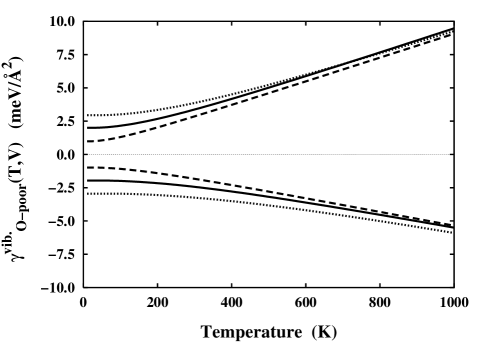
FIG. 1.: Vibrational contribution to the surface free energy, of a stoichiometric termination, cf. eq. (30), in the temperature range of interest to the present study. The Ru and O modes are approximated in the Einstein model by characteristic frequencies, $\bar{\omega}_{\rm O}^{\rm bulk}=80$ meV and $\bar{\omega}_{\rm Ru}^{\rm bulk}=$25 meV. Shown is the contribution, if the vibrational modes at the surface differed by $\pm 50$% from these bulk values (solid lines). To assess the dependence on the value chosen for the characteristic frequencies, the latter are varied by $\pm 50$% (dashed and dotted lines respectively). In all cases, the vibrational contribution stays below 10 meV/Ų in the whole temperature range considered.

Hence, we see that in the O-poor limit $\gamma_{\rm O-poor}^{\rm vib.}(T,p)$ of a stoichiometric termination arises primarily out of the difference of the vibrational modes at the oxide surface with respect to their bulk value. To arrive at numbers, we use $\bar{\omega}_{\rm O}^{\rm bulk}=80$ meV and $\bar{\omega}_{\rm Ru}^{\rm bulk}=$25 meV [8, 9], and allow a 50% variation of these values at the surface, to plot eq. (30) in Fig. 1 in the temperature range of interest to our study. As these particular values for the characteristic frequencies are not well justified, but should only be considered as rough estimates, we also include in the graph the corresponding $\gamma_{\rm O-poor}^{\rm vib.}(T,p)$, if these values changed by $\pm 50$%. From Fig. 1 we see that the vibrational contribution to the surface free energy stays within 10 meV/Ų in all of the considered cases, and that the uncertainty in the characteristic frequencies translates primarily to variations of $\gamma_{\rm O-poor}^{\rm vib.}(T,p)$ at low temperatures, where the value of the latter is very small anyway.

We have also computed the vibrational contribution to the surface free energy of non-stoichiometric terminations in an analogous manner. There, the formulas turn out more lengthy, cf. eq. (15), and the vibrational contribution includes not only differences between bulk and surface vibrational modes, but also absolute $F^{\rm vib.}(T,\omega)$ terms due to the excess or deficient atoms. Yet, even then the vibrational contribution stays within $\pm 10$ meV/Ų similar to the above described stoichiometric case. In conclusion, we therefore take this value to represent a good upper bound for the vibrational influence on the surface free energy.

Such a $\pm 10$ meV/Ų contribution is certainly not a completely negligible factor, yet as we will show below it is of the same order as the numerical uncertainty in our calculations. Furthermore, as will become apparent in the discussion of the results, this uncertainty does not affect any of the physical conclusions drawn in the present application. Hence, we will henceforth neglect the complete vibrational contribution to the Gibbs free energy, leaving only the total energies $E^{\rm total}(V,N_{\rm Ru},N_{\rm O})$ as the predominant term. In turn, this allows us to rewrite eq. (15) to

$$\gamma_{\rm O-poor}(T,p)\approx\frac{1}{2A}\bigg{[}\;E^{\rm slab}(V,N_{\rm Ru},N_{\rm O})\;-$$ (33)

$$\left.\frac{N_{\rm O}}{2}E^{\rm bulk}_{\rm RuO_{2}}(V)-\left(N_{\rm Ru}-\frac{N_{\rm O}}{2}\right)E^{\rm bulk}_{\rm Ru}(V)\right],$$ (34)

which now contains exclusively terms directly accessible to a DFT calculation. We stress, that this approximation is well justified in the present case, but it is not a general result: There might well be applications, where the inclusion of vibrational effects on the surface free energy can be crucial.

E Pressure and temperature dependence of $\mu_{\rm O}(T,p)$

Having completely described the recipe of how to obtain $\gamma(T,p)$ as a function of the O chemical potential, the remaining task is to relate the latter to a given temperature, $T$, and pressure, $p$. As the surrounding O₂ atmosphere forms an ideal gas like reservoir, we can obtain in the appendix the following expression

$$\mu_{\rm O}(T,p)=\mu_{\rm O}(T,p^{\circ})\;+\;1/2\;kT\;ln\left(\frac{p}{p^{\circ}}\right),$$ (35)

which already gives us the temperature and pressure dependence, if we only know the temperature dependence of $\mu_{\rm O}(T,p^{\circ})$ at one particular pressure, $p^{\circ}$.

TABLE I.: $\mu_{\rm O}(T,p^{\circ})$ in the temperature range of interest to our study. The entropy and enthalpy changes used to obtain $\mu_{\rm O}(T,p^{\circ})$ via eq. (38) are taken from the JANAF thermochemical tables at $p^{\circ}=1{\rm atm}$ [10].

$T$	$\mu_{\rm O}(T,p^{\circ})$	$T$	$\mu_{\rm O}(T,p^{\circ})$
100 K	-0.08 eV	600 K	-0.61 eV
200 K	-0.17 eV	700 K	-0.73 eV
300 K	-0.27 eV	800 K	-0.85 eV
400 K	-0.38 eV	900 K	-0.98 eV
500 K	-0.50 eV	1000 K	-1.10 eV

We choose as the zero reference state of $\mu_{\rm O}(T,p)$ the total energy of oxygen in an isolated molecule, i.e. $\mu_{\rm O}(0{\rm K},p)=1/2\;E^{\rm total}_{\rm O_{2}}\equiv 0$. With respect to this zero, reached at our theoretical oxygen-rich limit, cf. eq. (12), $\mu_{\rm O}(T,p^{\circ})$ is then given by

$$\mu_{\rm O}(T,p^{\circ}) = \mu_{\rm O}^{\rm O-rich}(0{\rm K},p^{\circ})\;+\;1/2\;\Delta G(\Delta T,p^{\circ},{\rm O_{2}})\;=$$ (38)

$$1/2\;\left(H(T,p^{\circ},{\rm O_{2}})-H(0{\rm K},p^{\circ},{\rm O_{2}})\right)\;-$$

$$1/2\;T\;\left(S(T,p^{\circ},{\rm O_{2}})-S(0{\rm K},p^{\circ},{\rm O_{2}})\right),$$

where we have used the relation $G=H-TS$ between the Gibbs free energy and the enthalphy, $H$. This allows us to obtain the aspired temperature dependence simply from the differences in the enthalpy and entropy of an O₂ molecule with respect to the $T=0$ K limit. For standard pressure, $p^{\circ}=$ 1 atm, these values are e.g. tabulated in the JANAF thermochemical tables [10]. Plugging them into eq. (38) leads finally to $\mu_{\rm O}(T,p^{\circ})$, which we list in Table I.

Together with eq. (35) the O chemical potential can thus be obtained for any given $(T,p)$ pair. Although we prefer to conveniently present the resulting surface energies as a one-dimensional function of $\mu_{\rm O}(T,p)$, we will often convert this dependence also into a temperature (pressure) dependence at a fixed pressure (temperature) in a second $x$-axis to elucidate the physical meaning behind the obtained curves.

F DFT basis set and convergence

The DFT input to eq. (33) has been obtained using the full-potential linear augmented plane wave method (FP-LAPW) [11, 12, 13] within the generalized gradient approximation (GGA) of the exchange-correlation functional [14]. For the RuO₂(110) surface calculation we use a symmetric slab consisting of 3 rutile O-(RuO)-O trilayers, where all atomic positions within the outermost trilayer were fully relaxed. A vacuum region of $\approx$ 11 Å is employed to decouple the surfaces of consecutive slabs in the supercell approach. Test calculations with 5 and 7 trilayered slabs, as well as with a vacuum region up to $\approx$ 28 Å confirmed the good convergence of this chosen setup with variations of $\gamma(T,p)$ smaller than $\pm$ 3 meV/Ų. Allowing a relaxation of deeper surface layers in the thicker slabs did not result in a significant variation of the respective atomic positions, nor did it influence the near-surface geometry as obtained in the calculations with the standard 3 trilayer slabs. To ensure maximum consistency, the corresponding RuO₂ bulk computations are done in exactly the same (110) oriented unit cell as used for the slabs, in which the prior vacuum region is simply replaced by additional RuO₂ trilayers.

The FP-LAPW basis set is taken as follows: $R_{\rm{MT}}^{\rm{Ru}}=$1.8 bohr, $R_{\rm{MT}}^{\rm{O}}=$1.3 bohr, wave function expansion inside the muffin tins up to $l_{\rm{max}}^{\rm{wf}}=12$, potential expansion up to $l_{\rm{max}}^{\rm{pot}}=4$. For the RuO₂(110) slabs the Brillouin zone integration was performed using a $(5\times 10\times 1)$ Monkhorst-Pack grid with 15 k-points in the irreducible part. The energy cutoff for the plane wave representation in the interstitial region between the muffin tin spheres was 17 Ry for the wave functions and 169 Ry for the potential. Checking on the convergence, the surface free energies of the three possible $(1\times 1)$ RuO₂(110) truncations discussed below were found unchanged to within 1 meV/Ų by increasing the k-mesh to a $(7\times 14\times 1)$ Monkhorst-Pack grid with 28 k-points in the irreducible part. A larger interstitial cutoff up to 24 Ry reduced the absolute values of the three $\gamma(T,p)$ by up to 10 meV/Ų, yet as all of them were reduced alike, their respective differences (which are the only relevant quantities entering the physical argument) stayed constant to within 5 meV/Ų.

In total we thus find the numerical accuracy of the calculated surface free energies with respect to the supercell approach and the finite basis set to be within 10 meV/Ų, which will not affect any of the physical conclusions drawn. Note, that the stated imprecision does not include possible errors introduced by more general deficiencies of the approach, namely the use of the GGA as exchange-correlation functional, on which we will comment below.

III Results

A RuO₂(110) surface structure

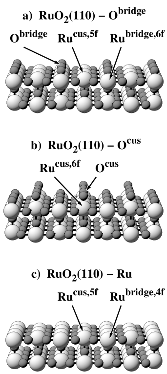
FIG. 2.: Three possible terminating planes of the rutile (110) surface: a) Stoichiometric RuO₂(110)-O^bridge termination with five-, six- and twofold coordinated Ru^cus,5f, Ru^bridge,6f and O^bridge atoms respectively. b) RuO₂(110)-O^cus termination, where additional O^cus atoms sit atop the formerly undercoordinated Ru^cus,6f atoms. c) RuO₂(110)-Ru termination, which lacks the O^bridge atoms in comparison to the stoichiometric termination (Ru = large, light spheres, O = small, dark spheres).

RuO₂ crystallizes in the rutile bulk structure, in which every metal atom is coordinated to six oxygens, and every oxygen to three metal neighbors [15]. The oxygens forming an octahedron around each Ru atom are not all equivalent, but can be distinguished into four basal and two apical O atoms with calculated O-Ru bondlengths of 2.00 Å and 1.96 Å respectively. We notice that along the (110) direction this structure can then be viewed as a stacking sequence of O-(RuO)-O trilayers, in which each trilayer is simply composed of an alternating sequence of in-plane and up-right oriented oxygen-ruthenium coordination octahedra, cf. Fig. 2b. Cut along (110), the rutile bulk structure can therefore exhibit three distinct terminations of $(1\times 1)$ periodicity, depending at which plane the trilayer is truncated, cf. Fig. 2a-c.

Traditionally, the stoichiometric RuO₂(110)-O^bridge termination is believed to be the most stable one for all (110) surfaces of rutile-structured crystals [4, 5], as in the ionic model it leads to an uncharged surface and cuts the least number of bonds: While the Ru^bridge,6f atoms possess their ideal sixfold O coordination with two of their basal oxygens forming the terminal O^bridge atoms, only the Ru^cus,5f lack one apical on-top O, cf. Fig. 2a. Note, that we will use a nomenclature for the surface Ru atoms, where apart from a site specific characterization (e.g. cus for the coordinatively unsaturated site in the stoichiometric termination) also the number of direct O neighbors (e.g. 5f for 5-fold coordination) is stated. Vice versa, we indicate for the surface O atoms to which specific site they bind (e.g. O^bridge binds to the Ru^bridge,6f atoms).

Alternatively, in the second possible RuO₂(110)-O^cus termination, cf. Fig. 2b, terminal O^cus atoms occupy sites atop of the formerly undercoordinated Ru^cus,6f atoms, so that now all metal atoms in the surface possess their ideal sixfold coordination. This is, of course, paid for by the presence of both the only twofold and onefold coordinated O^bridge and O^cus atoms, respectively. Finally, the third RuO₂(110)-Ru termination exhibiting the mixed (RuO) plane at the surface is achieved by removing the O^bridge atoms from the stoichiometric termination, cf. Fig. 2c. Here, no undercoordinated oxygens are present any more, yet, at the expense of the four- and fivefold bonded Ru^bridge,4f and Ru^cus,5f atoms.

B Prediction of a high pressure termination

FIG. 3.: Surface free energies, $\gamma(T,p)$, of the three RuO₂(110) terminations depicted in Fig. 2. Additionally shown as dashed line is the surface free energy of a RuO₂(110)-O^cus termination, in which only every second O^cus site along the trenches is occupied. The dotted vertical lines indicate the allowed range of the oxygen chemical potential, $\mu_{\rm O}(T,p)$, using $1/2\;E^{\rm total}_{\rm O_{2}}$ as zero reference as explained in Section IIB. In the top $x$-axis, the dependence on $\mu_{\rm O}(T,p)$ has been cast into a pressure scale at a fixed temperature of $T=$ 600 K.

The calculated surface free energies of the three possible terminations are shown in Fig. 3. As explained in connection with eq. (19), the RuO₂(110)-O^cus (RuO₂(110)-Ru) termination with an excess (deficiency) of O at the surface becomes more and more favorable (unfavorable) towards the O-rich limit, while the stoichiometric RuO₂(110)-O^bridge termination exhibits a constant $\gamma(T,p)$. Indeed, we find the traditionally assumed stoichiometric RuO₂(110)-O^bridge surface to be the most stable over quite a range of oxygen chemical potentials above the O-poor limit. To make this range a bit more lucid, we have used eq. (35) to convert $\mu_{\rm O}(T,p)$ into a physically more comprehensible pressure dependence at a fixed temperature, cf. the top $x$-axis of Fig. 3. The temperature of $T=600$ K corresponds to a typical annealing temperature employed experimentally for this system [9, 16, 17, 18, 19]. From the resulting pressure scale we see, that the stability of the stoichiometric termination extends therefore roughly around the pressure range corresponding to UHV conditions.

Yet, this is different at higher O pressures, where the RuO₂(110)-O^cus termination becomes the most stable surface structure, cf. Fig. 3. In the O-rich limit, it exhibits a $\gamma^{\rm O-rich}(T,p)$, which is by 49 meV/Ų lower than the one of the stoichiometric RuO₂(110)-O^bridge surface, i.e. the deduced crossover between the two terminations is far beyond the estimated uncertainty of $\approx\pm 10$ meV/Ų due to the neglection of the vibrational contribution to the Gibbs free energies and due to the finite basis set. This estimate does, however, not comprise the more general error due to the use of the GGA as exchange-correlation functional. To this end, we have also calculated the surface free energies of the two competing terminations within the local density approximation (LDA) [20]. Although the absolute values of both $\gamma^{\rm O-poor}(T,p)$ turn out to be by $\approx$ 15 meV/Ų higher, their respective difference is almost unchanged, which is eventually what determines the crossover point of the two lines in Fig. 3. The RuO₂(110)-O^cus termination is therefore the lowest energy structure for $\mu_{\rm O}(T,p)>-0.85$ eV in the LDA, which is almost the same as the $\mu_{\rm O}(T,p)>-0.93$ eV found with the GGA, shown in Fig. 3. Consequently, while the choice of the exchange-correlation functional may affect the exact transition temperature or pressure, the transition per se is untouched. In turn, we may safely predict the stability of a polar surface termination on RuO₂(110) at high O chemical potential, corresponding e.g. to the pressure range typical for catalytic applications.

Note, that Fig. 3 summarizes only the $\gamma(T,p)$ of the three $(1\times 1)$ terminations, which arise by truncating the RuO₂ crystal at bulk-like planes in the (110) orientation. Yet, it is a priori not clear, that the terminal atoms at the surface must be in the sites corresponding to the bulk stacking sequence. To check this, we have additionally calculated the surface free energies of surface structures, where the O^bridge (O^cus) atoms occupy atop (bridge) sites over the Ru^bridge,5f (Ru^cus,6f) atoms, instead of their normal bridging (atop) configuration. In both cases, we find the $\gamma(T,p)$ considerably higher, which excludes the possibility that these adatoms occupy non bulk-like sites at the surface. Similarly, a RuO₂(110)-O^cus termination, where the O^bridge atoms have been removed, can also safely be ruled out as alternative for a stoichiometrically terminated surface.

C Lateral interaction between O^cus atoms and vacancy concentration

The reasoning of the last Section leaves in fact only the RuO₂(110)-O^bridge and RuO₂(110)-O^cus termination as the relevant surface structures stabilized in UHV and under high O pressure respectively. Both differ from each other only by the presence of the additional O^cus atoms, which continue the bulk stacking sequence by filling the vacant sites atop of the formerly undercoordinated Ru^cus,5f atoms. The way the RuO₂(110)-O^cus termination is formed at an increasing oxygen chemical potential will therefore depend significantly on the details of the lateral interaction among this adatom species.

The RuO₂(110)-O^bridge surface has a trench-like structure with a distance of 6.43 Å between the rows formed by the O^bridge atoms, cf. Fig. 2a. This renders any lateral interaction between O^cus atoms adsorbed in neighboring trenches rather unlikely. On the other hand, the distance between two O^cus atoms occupying neighboring sites along one trench is only 3.12 Å. To check on the corresponding interaction we calculated the surface free energy of a RuO₂(110)-O^cus termination in a $(2\times 1)$ supercell, in which the O^cus atoms occupied only every other site along the trenches. The corresponding $\gamma(T,p)$ is drawn as a dashed line in Fig. 3. As now only half of the excess O^cus atoms are present, the slope of this curve has to be one half of the slope of the line representing the normal RuO₂(110)-O^cus termination, cf. eq. (19).

Interestingly, both curves cross the stoichiometric RuO₂(110)-O^bridge line in exactly the same point. This can only be understood by assuming a negligible lateral interaction between neighboring O^cus atoms: If there was an attractive (repulsive) interaction between them, then it would be favorable (unfavorable) to put O^cus atoms as close to each other as possible. In turn, the $(2\times 1)$ overlayer of O^cus atoms, in which only every other site is occupied, would be less (more) stable than the normal RuO₂(110)-O^cus termination, where all neighboring sites are full. Consequently, the stability with respect to the stoichiometric termination would be decreased (enhanced), leading to a later (earlier) crossover point in Fig. 3. That both calculated lines cross the RuO₂(110)-O^bridge line at the same point is therefore a reflection of a negligible lateral interaction between the O^cus atoms.

Additionally, we compute a very high barrier of almost 1.5 eV for diffusion of O^cus atoms along the trenches, indicating that the latter species will be practically immobile in the temperature range, where the oxide is stable. This together with the small lateral interaction indicates that at increasing O chemical potential the RuO₂(110)-O^cus surface is formed from the stoichiometric termination by a random occupation of O^cus sites, until eventually the whole surface is covered. Not withstanding, at finite temperatures there will still be a certain vacancy concentration even at O chemical potentials above the crossover point of the two terminations. As the undercoordinated Ru^cus,5f atoms exposed at such a vacant O^cus site, cf. Fig. 2, might be chemically active sites for surface reactions [18], it is interesting to estimate how many of these sites will be present under given $(T,p)$ conditions.

Since we have shown that each O^cus site at the surface is filled independently from the others, we can calculate its occupation probability within a simple two level system (site occupied or vacant) in contact with a heat bath. The vacancy concentration follows then from a canonic distribution, where the energy of the two levels is given by the $\gamma(T,p)$ of the two terminations at the chosen chemical potential. As an example, we first address room temperature, where the RuO₂(110)-O^cus termination becomes stable at pressures higher than $p\sim 10^{-22}$ atm. A vacancy concentration of only $1\%$ is in turn already reached at $p\sim 10^{-17}$ atm, so that at this temperature there will only be a negligible number of vacancies on the O^cus-terminated surface for any realistic pressure.

However, this situation becomes completely different at elevated temperatures. At $T=800$ K, the crossover to the RuO₂(110)-O^cus-termination occurs at $p\sim 10^{-1}$ atm with a $10\%$ vacancy concentration still present at 10² atm. In the range of atmospheric pressures the RuO₂(110) surface will therefore exhibit a considerable number of vacancies, which could explain the high catalytic activity reported for this material [18, 19, 21, 22, 23, 24]. However, although we have deliberately chosen $T=800$ K as a typical catalytic temperature, where e.g. a maximum conversion rate for the CO/CO₂ oxidation reaction over RuO₂(110) was found [22], we immediately stress that our reasoning is at the moment only based on the O pressure alone and therefore not directly applicable to catalysis experiments, which may also depend on the partial pressure of other reactants in the gas phase.

D On the stability of polar surfaces

As already mentioned in the introduction, the predicted high pressure RuO₂(110)-O^cus termination is traditionally not expected as it forms a so-called polar surface, which should not be stable on electrostatic grounds [4, 5]. The corresponding argument is based on the ionic model of oxides, in which every atom in the solid is assumed to be in its bulk formal oxidation state. Along a particular direction, $z$, the crystal may then be viewed as a stack of planes with charge $q$, each of which contribute with $V(z)\propto qz$ to the total electrostatic potential. As this contribution diverges at infinite distances the crystal as a whole can in turn only be stable, if constructed as a neutral block, in which all infinities due to the individual planes cancel. For RuO₂(110), which is a type 2 surface in Tasker’s widely used classification scheme [25], the only neutral repeat unit is a symmetric O-(RuO)-O trilayer with a (-2)-(+4)-(-2) charge sequence, so that the only surface termination without net dipole moment would correspondingly be the stoichiometric RuO₂(110)-O^bridge termination.

FIG. 4.: Surface free energies, $\gamma(T,p)$, of the stoichiometric RuO₂(110)-O^bridge and polar RuO₂(110)-O^cus termination. Shown is the effect of relaxation at the surface, with solid lines indicating fully relaxed surface structures and dashed lines the corresponding bulk-truncated geometries. The dependence on the oxygen chemical potential has been translated into a temperature scale at $10^{-12}$ atm (bottom $x$-axis) and 1 atm (top $x$-axis) pressure.

On the other hand, the RuO₂(110)-O^cus termination with its extra unmatched (-2) charge plane formed by the O^cus atoms would lead to a diverging potential and should thus not be stable. That we indeed find this surface stabilized at higher O chemical potentials points to the most obvious shortcoming of the electrostatic model, namely the assumption that all atoms in the solid are identical, i.e. that also all surface atoms are both structurally as well as electronically in a bulk-like state. In how much already the additional structural degrees of freedom at the surface influence the stability is exemplified in Fig. 4, where the surface free energies of the two relevant terminations are compared in either a bulk-truncated or the fully relaxed geometry. While the small relaxation of the RuO₂(110)-O^bridge termination hardly affects the $\gamma(T,p)$, the bulk-truncated RuO₂(110)-O^cus surface turns out considerably less stable compared to its relaxed counterpart. The by +2.5 eV strongly increased workfunction of the bulk-truncated RuO₂(110)-O^cus surface with respect to the stoichiometric termination shows that the addition of the O^cus atoms indeed induces a considerable dipole moment as suggested by the ionic model. Yet, just the relaxation lowers this workfunction again by 1 eV, indicating that the dipole moment can already be considerably reduced via a strongly shortened O^cus-Ru^cus,6f bondlength of 1.70 Å (compared to the bulk-like 1.96 Å), therewith considerably stabilizing the surface.

FIG. 5.: ($x,y$)-averaged Kohn-Sham effective, $V^{\rm eff}(z)$ (dashed line), and electrostatic potential, $V^{\rm es}(z)$ (solid line), along the (110) direction perpendicular to the surface, $z$. Additionally shown is the workfunction, $\Phi$, as dotted line. a) Bulk-truncated RuO₂(110)-O^bridge termination ($\Phi=5.7$ eV), b) Bulk-truncated RuO₂(110)-O^cus termination ($\Phi=8.2$ eV), and c) Fully relaxed RuO₂(110)-O^cus termination ($\Phi=7.2$ eV). The top $x$-axis marks the position of O-(RuO)-O layers in the crystal.

Yet, not only structurally, but also electronically the topmost layers in the RuO₂(110)-O^cus surface differ appreciably from their respective bulk counterparts. This is illustrated in Fig. 5, where we show the ($x,y$)-averaged potential along the (110) direction perpendicular to the surface, $z$. In the bulk-truncated, stoichiometric RuO₂(110)-O^bridge termination in Fig. 5a the electrostatic potential at the topmost O-(RuO)-O trilayer is still almost identical to the corresponding one in the deeper trilayers, thus enabling in this case a description of this surface in terms of bulk-like planes as assumed in the ionic model. On the contrary, we find a significant deviation of the potential in the outermost layers of the RuO₂(110)-O^cus termination, cf. Fig. 5b, even for a bulk-truncated geometry. This difference is further enhanced by the structural relaxation, cf. Fig. 5c, so that the topmost (RuO)-O-O planes of this termination are certainly not well characterized by bulk properties, thus invalidating the electrostatic argument raised against this polar surface.

Instead, we argue that the surface fringe composed by the topmost layers should be viewed as a new material, which properties might differ considerably from the bulk stacking sequence due to the additional structural and electronic degrees of freedom present at the surface. A similar conclusion has previously been reached by Wang et al. [2, 3], who discussed the stability of oxygen-terminated polar (0001) surfaces of corundum-structured $\alpha$-Fe₂O₃ and $\alpha$-Al₂O₃. This indicates, that the traditionally dismissed polar terminations [6] might indeed be a more general phenomenon, which existence could be a crucial ingredient to understand the function of oxide surfaces under realistic environmental conditions. As particularly polar terminations with excess oxygen can be stabilized at increased O₂ partial pressure in the gas phase, the different properties of the latter should be taken into consideration, when modelling high pressure applications like catalysis.

E Importance of experimental preparation conditions

This influence of the O₂ partial pressure on the surface morphology and function has recently become apparent in a number of studies addressing the reported high CO oxidation rates over Ru catalysts. While it was for a long time believed that the active species is the Ru metal itself [26, 27, 28, 29], the decisive role played by oxide patches formed under catalytic conditions was only recently realized [17, 18, 19, 21, 22]. This was primarily due to the problem of preparing a fully oxidized surface in a controlled manner under UHV conditions. Yet, by means of more oxidizing carrier gases or higher O partial pressures it is now possible to circumvent this materials gap [30], enabling the detailed characterization of RuO₂(110) domains formed on the model Ru(0001) surface with the techniques of surface science [9, 17, 18, 19, 21, 22, 23, 24].

However, the results of the present study show that the surface termination of these domains changes with the O₂ pressure, too. Not aware of this dependence a reaction mechanism for the CO oxidation was previously proposed, situated solely on the stoichiometric RuO₂(110)-O^bridge termination that was characterized in the respective LEED study under UHV conditions [18, 19]. While it is presently not clear, to what extent the O^cus atoms additionally present under catalytic pressures are involved in the reaction [23, 24], this still highlights the delicacy with which the results of UHV spectroscopies and post-exposure experiments have to be applied to model catalysis and steady-state conditions.

Only very recently UHV studies achieved to stabilize the high-pressure RuO₂(110)-O^cus termination intentionally by postdosing O₂ at low temperatures [9, 17, 23, 24]. Temperature desorption spectroscopy (TDS) experiments found the corresponding excess O^cus atoms to be stable up to about 300-550 K in UHV [17]. This agrees nicely with the calculated transition temperature of $450\pm 50$ K at the crossover point between the two terminations for a pressure of $10^{-12\pm 2}$ atm, presumably present during a typical TDS experiment [31], cf. the bottom $x$-axis of Fig. 4. Yet, the actual desorption temperature is of course significantly higher for the orders of magnitude higher O₂ partial pressures present in catalytic applications. This is exemplified by the temperature scale on the top $x$-axis of Fig. 4 at a pressure of $p=1$ atm, representative for the early high-pressure experiments addressing the high CO/CO₂ conversion rates of Ru catalysts [27, 28]. The corresponding elevated transition temperature of 900 K shows that O^cus atoms were most probably present on oxidized RuO₂(110) domains in all of these experiments.

The presence of the hitherto unaccounted high-pressure termination of RuO₂(110) might therefore be an essential keystone to understand the data obtained from grown RuO₂(110) films or oxidized Ru(0001) surfaces, which are unanimously prepared under highly O-rich conditions. We already exemplified this in a preceding publication [32] by suggesting that the long discussed, largely shifted satellite peak in Ru $3d$ x-ray photoemission spectroscopy (XPS) data from such surfaces [16, 33], is due to the Ru^cus,6f atoms in the RuO₂(110)-O^cus termination, which experience a significantly different environment due to the aforementioned, very short bondlength to the O^cus atoms.

If the high-pressure termination created during the preparation of the crystal is frozen in during the transfer to UHV depends then on the details of the transfer itself, e.g. on such nitty-gritties of whether or not the temperature is kept constant while the pressure goes down to its base value after exposure. A dependence of the TDS data of an oxygen-rich Ru(0001) surface on these parameters has already been reported and considered by Böttcher and Niehus [17], while the final annealing step to 600 K after transfer to UHV employed in the LEED work identifying RuO₂(110) domains on oxidized Ru(0001) [18, 19] explains, why there only the stoichiometric RuO₂(110)-O^bridge termination could be characterized, cf. Fig. 3.

Such dependences on the experimental preparation have hitherto often been neglected, entailing only a low comparability of data sets obtained in different groups. Instead, the present results demonstrate that systematic investigations in the whole $(T,p)$ range are required to fully identify the surface structure and composition of oxide surfaces at realistic conditions, which in turn is a prerequisite before tackling the long-term goal of understanding the function of the latter in the wealth of everyday applications.

IV Summary

In conclusion we have combined density-functional theory (DFT) and classical thermodynamics to determine the lowest energy structure of an oxide surface in equilibrium with an O environment. The formalism is applied to RuO₂(110) showing that apart from the expected stoichiometric surface, a so-called polar termination with an excess of oxygen (O^cus) is stabilized at high O chemical potentials. Depending on the details of the experimental preparation conditions, either of the two terminations can therefore be present, which different properties have to be taken into account, when trying to understand the obtained data or aiming to extrapolate the results of UHV ex situ techniques to high-pressure applications like oxidation catalysis.

A polar termination is traditionally not conceived to be stable within the framework of electrostatic arguments based on the ionic model of oxides. We show that this reasoning is of little validity as it assumes all atoms to be in the same bulk-like state. On the contrary, the additional structural and electronic degrees of freedom at an oxide surface allow substantial deviations from these bulk properties and may thus stabilize even non-stoichiometric surface terminations. A similar conclusion was previously reached also for the O-rich (0001) termination of corundum-structured $\alpha$-Fe₂O₃ indicating that polar surfaces might indeed be a more general feature of transition metal oxides. The concentration of oxygen vacancies found for the polar termination of RuO₂(110) at atmospheric pressures and elevated temperatures could finally possibly explain the high catalytic activity reported for this surface.

A

1 Vibrational contribution to the Gibbs free energy

The vibrational contribution to the Gibbs free energy comprises vibrational energy and entropy, cf. eq. (24). Both can be calculated from the partition function of an $N$-atomic system [34]

$$Z\;=\;\sum_{i=1}^{3N}\int\frac{d{\bf k}}{(2\pi)^{3}}\;\sum_{n=0}^{\infty}e^{-(n+\frac{1}{2})\beta\hbar\omega_{i}({\bf k})},$$ (A1)

where $\beta=1/kT$ and the $\omega_{i}({\bf k})$ are the $3N$ vibrational modes. The vibrational energy is then given by

$$E^{\rm vib.}(T,V,N)\;=\;-\frac{\partial}{\partial\beta}lnZ,$$ (A2)

and the entropy is defined as

$$S^{\rm vib.}(T,V,N)\;=\;k\left(\;lnZ\;+\;\beta E^{\rm vib.}\;\right).$$ (A3)

Writing $F^{\rm vib.}(T,V,N)$ as a frequency integral including the phononic density of states, $\sigma(\omega)$, and using the relation $F^{\rm vib.}=E^{\rm vib.}-TS^{\rm vib.}$, one arrives at

$$F^{\rm vib.}(T,\omega) = \hbar\omega\left(\frac{1}{2}\;+\;\frac{1}{e^{\beta\hbar\omega}-1}\right)\;-$$ (A5)

$$kT\left[\frac{\beta\hbar\omega}{e^{\beta\hbar\omega}-1}\;-\;ln\left(1-e^{-\beta\hbar\omega}\right)\right].$$

2 Ideal gas expression for $\mu_{O_{2}}(T,p)$

For an ideal gas of $N$ particles at constant pressure, $p$, and temperature, $T$, the chemical potential is simply given by the Gibbs free energy per atom,

$$\mu\;=\;\left(\frac{\partial G}{\partial N}\right)_{T,p,N}\;=\;\frac{G}{N}.$$ (A6)

As the Gibbs free energy is a potential function depending on pressure and temperature, its total derivative can be written as

$$dG = \left(\frac{\partial G}{\partial T}\right)_{p}dT\;+\;\left(\frac{\partial G}{\partial p}\right)_{T}dp\;=$$ (A8)

$$-SdT\;+\;Vdp,$$

where we have inserted the Maxwell relations for the entropy, $S$, and volume, $V$. Using the ideal gas equation of state, $pV=NkT$, the partial derivative of $G(T,p)$ with respect to pressure at constant temperature is consequently

$$\left(\frac{\partial G}{\partial p}\right)_{T}\;=\;V\;=\;\frac{NkT}{p}.$$ (A9)

In turn, a finite pressure change from $p$ to $p^{\circ}$ results in

$$G(T,p)-G(T,p^{\circ}) = \int_{p^{\circ}}^{p}\;\left(\frac{\partial G}{\partial p}\right)_{T}dp\;=$$ (A11)

$$NkT\;ln\left(p/p^{\circ}\right).$$

Combining eqs. (A6) and (A11), we can finally write for the chemical potential of O

$$\mu_{\rm O}(T,p) = 1/2\;\mu_{\rm O_{2}}(T,p)\;=$$ (A12)

$$= \mu_{\rm O}(T,p^{\circ})\;+\;1/2\;kT\;ln\left(p/p^{\circ}\right),$$ (A13)

which is the expression used in Section IIE.

REFERENCES

- [1] C. Stampfl, M.V. Ganduglia-Pirovano, K. Reuter, and M. Scheffler, Surf. Sci. 500, (accepted); preprint download under http://www.fhi-berlin.mpg.de/th/pub01.html.
- [2] X.-G. Wang, W. Weiss, Sh.K. Shaikhutdinov, M. Ritter, M. Petersen, F. Wagner, R. Schlögl, and M. Scheffler, Phys. Rev. Lett. 81, 1038 (1998).
- [3] X.-G. Wang, A. Chaka, and M. Scheffler, Phys. Rev. Lett. 84, 3650 (2000).
- [4] V.E. Henrich and P.A. Cox, The Surface Science of Metal Oxides, Cambridge University Press, Cambridge (1994).
- [5] C. Noguera, Physics and Chemistry at Oxide Surfaces, Cambridge University Press, Cambridge (1996).
- [6] C. Noguera, J. Phys. Cond. Mat. 12, R367 (2000).
- [7] CRC Handbook of Chemistry and Physics, 76th ed. (CRC Press, Boca Raton FL, 1995).
- [8] R. Heid, L. Pintschovius, W. Reichardt, and K.-P. Bohnen, Phys. Rev. B 61, 12059 (2000).
- [9] Y.D. Kim, A.P. Seitsonen, S. Wendt, J. Wang, C. Fan, K. Jacobi, H. Over, and G. Ertl, J. Phys. Chem. 105, 3752 (2001).
- [10] D.R. Stull and H. Prophet, JANAF Thermochemical Tables, 2nd ed., U.S. National Bureau of Standards, Washington, D.C. (1971).
- [11] P. Blaha, K. Schwarz and J. Luitz, WIEN97, A Full Potential Linearized Augmented Plane Wave Package for Calculating Crystal Properties, Karlheinz Schwarz, Techn. Universität Wien, Austria, (1999). ISBN 3-9501031-0-4.
- [12] B. Kohler, S. Wilke, M. Scheffler, R. Kouba, and C. Ambrosch-Draxl, Comput. Phys. Commun. 94, 31 (1996).
- [13] M. Petersen, F. Wagner, L. Hufnagel, M. Scheffler, P. Blaha, and K. Schwarz, Comp. Phys. Commun. 126, 294 (2000).
- [14] J.P. Perdew, K. Burke and M. Ernzerhof, Phys. Rev. Lett. 77, 3865 (1996).
- [15] P.I. Sorantin and K.H. Schwarz, Inorg. Chem. 31, 567 (1992).
- [16] Lj. Atanasoska, W.E. O’Grady, R.T. Atanasoski, and F.H. Pollak, Surf. Sci. 202, 142 (1988).
- [17] A. Böttcher and H. Niehus, Phys. Rev. B 60, 14396 (1999).
- [18] H. Over, Y.D. Kim, A.P. Seitsonen, S. Wendt, E. Lundgren, M. Schmid, P. Varga, A. Morgante, and G. Ertl, Science 287, 1474 (2000).
- [19] Y.D. Kim, H. Over, G. Krabbes, and G. Ertl, Topics in Catalysis 14, 95 (2001).
- [20] J.P. Perdew and Y. Wang, Phys. Rev. B 45, 13244 (1992).
- [21] A. Böttcher, H. Niehus, S. Schwegmann, H. Over, and G. Ertl, J. Phys. Chem. B 101, 11185 (1997).
- [22] A. Böttcher, H. Conrad, and H. Niehus, Surf. Sci. 452, 125 (2000).
- [23] C.Y. Fan, J. Wang, K. Jacobi, and G. Ertl, J. Chem. Phys. 114, 10058 (2001).
- [24] J. Wang, C.Y. Fan, K. Jacobi, and G. Ertl, Surf. Sci. 481, 113 (2001).
- [25] P.W. Tasker, J. Phys. C 12, 4977 (1979).
- [26] T.E. Madey, H.A. Engelhardt, and D. Menzel, Surf. Sci. 48, 304 (1975).
- [27] N.W. Cant, P.C. Hicks, and B.S. Lennon, J. Catal. 54, 372 (1978).
- [28] C.H.F. Peden and D.W. Goodman, J. Phys. Chem. 90, 1360 (1986).
- [29] C. Stampfl, S. Schwegmann, H. Over, M. Scheffler, and G. Ertl, Phys. Rev. Lett. 77, 3371 (1996).
- [30] A. Böttcher and H. Niehus, J. Chem. Phys. 110, 3186 (1999).
- [31] A TDS experiment with a low heating rate of 6 K/s is considered to refer to a situation, where the system is always close to equilibrium. Indeed, the agreement of the experimental results of Böttcher and Niehus [30] with our calculations confirmes this assumption.
- [32] K. Reuter and M. Scheffler, Surf. Sci. (in press).
- [33] Y.J. Kim, Y. Gao, and S.A. Chambers, Appl. Surf. Sci. 120, 250 (1997); and references therein.
- [34] N.W. Ashcroft and N.D Mermin, Solid State Physics, CBS Publishing, Tokio (1981).