[

Statistical Features of Drainage Basins in Mars Channel Networks.

Abstract

Erosion by flowing water is one of the major forces shaping the surface of Earth. Studies in the last decade have shown, in particular, that the drainage region of rivers, where water is collected, exhibits scale invariant features characterized by exponents that are the same for rivers around the world. Here we show that from the data obtained by the MOLA altimeter of the Mars Global Surveyor one can perform the same analysis for mountain sides on Mars. We then show that in some regions fluid erosion might have played a role in the present martian landscape.

]

Whether water flowed on the surface of Mars in the past is one of the most intriguing and challenging problems of contemporary planetary science. Indeed the presence of surface water, even some billion years ago, would make the odds for the development of life (as we know it) on Mars much higher. At present, the atmospheric conditions are almost incompatible with surface liquid water, so that its presence in the past has to be detected indirectly, looking at clues in the geomorphology of the planet. Moreover, understanding where water could have been present in the past is of great importance to choose the landing sites of future automatic and manned missions to Mars. Already early pictures taken from orbit showed canyons and channels similar to the ones carved by rivers on Earth. More recently, the high resolution pictures taken in the last three years by the Mars Orbiter Camera (MOC) camera of the NASA probe Mars Global Surveyor (MGS) have provided a wealth of data that add some more clues: gullies on the walls of craters and valleys [1], that suggest the presence of liquid water in (geologically) recent times, sedimentary rock formations typical, on Earth, of the beds of ancient lakes [2], the presence of an ocean in the northern hemisphere [3] and rootless cones similar to the ones that are found on Earth where molten lava has flowed over waterlogged ground[4]. All these photographic evidence needs to be complemented by some more robust analysis on data such as the ones from the Mars Orbiter Laser Altimeter (MOLA). Here we show that the channel networks that can be inferred from the MOLA data bear similarities with the structures carved by water erosion on Earth.

On Earth fluvial systems can be described through the self-affine properties of their drainage basin, where water, either from underground sources or from rain, is collected [5, 6]. Those self-affine properties have been established starting from Hack’s seminal work where the scaling relation (1) between the basin area $A$ and the length $L_{\parallel}$ of the basin’s main stream was proposed [7]:

$$A^{h}\sim L_{\parallel}$$ (1)

¿From measures on real rivers, the Hack’s exponent $h$ takes values between $0.5$ and $0.7$. The allometric relation between $A$ and $L_{\parallel}$ is just one in a number of scaling properties of drainage basins. In general, the drainage basin is characterized by the longitudinal length $L_{\parallel}$ (we use the same symbol as for the main stream length since, for real rivers, they scale in the same way) and by the transverse one, $L_{\perp}$ in such a way that $L_{\perp}\sim L_{\parallel}^{H}$. If the exponent $H$ is less than $1$, the basin is self-affine (the width of the basin scales slower than its length). If the basin is self-similar $H$ is equal to $1$ (the trivial case where the width scales as the length). The two exponents $H$ and $h$ are connected, as it is easy to see by comparing $L_{\perp}\sim L_{\parallel}^{H}$ together with Hack’s law (1): one finds that $h=1/(1+H)$. These two macroscopic features are not the only ones available in the study of drainage basins. In order to describe even more precisely the statistical properties channel networks, geomorphologists use Digital Elevation Models (DEM) [8, 9]. Measures, either ground based or, in more recent times, by satellites, provide the average height of an area that, on Earth, can be as little as $30\times 30m^{2}$. Each of these square units is associated to a pixel on an image (or, technically, to a site on a two dimensional square grid). Then, water collected in each pixel flows toward the lowest of the neighbor pixels, according to a simple maximal slope rule (other rules would be also viable, such as, for example, that water flows toward more than a single neighbor, and is partitioned proportionally to the slopes). If the maximal slope rule is applied, this procedure produces a branched structure without loops that should reproduce the visible river network. In a loopless branched structure, it is easy to define the region upstream of a given point, that is, the region whose collected water will all flow to that point. Therefore it is possible to label each and every point on the map by the area $A$ of its own drainage basin. The final outlet is of course labeled by the whole area of the basin. It is possible to draw the histogram of these areas for a given basin, finding that the frequency $P(A)$ to find a sub-basin of area $A$ follows the law $P(A)\sim A^{-\tau}$, where $\tau=1.43-1.46$. On the same branched structure, it is possible to measure the upstream length $L$ from a given point, as the distance of that point from the furthest source (a source is defined as a point without any upstream basin, that is, that does not collect any upstream water). Again, these lengths can be organized in a histogram, whose asymptotic behavior for the frequency distribution $\Pi(L)$ behaves as $\Pi(L)\sim L^{-\gamma}$, where $\gamma=1.7-1.8$. All these exponents, and others that could be defined, depend on the above exponent $H$ relating $L_{\perp}$ and $L_{\parallel}$, and then depend ultimately on the fractal properties of the basin. Using finite size scaling arguments, Maritan et al. [10] have shown that $\tau=2-h$, and $\gamma=1/h$. These relations hold for any kind of branched structure, whatever its origin, and they show that indeed there is only one independent exponent that determines all the others. Actually, one more independent exponent is the fractal dimension of the main stream; yet, river networks are, on the average, directed because water flows down slopes, which gives a preferential direction. Consequently the fractal dimension of the main stream is $d_{l}=1$. Still, the relations do not tell why the exponents should take a particular set of values. One can study the same statistical properties on a random landscape. In this case of course, due to the nature of the landscape, many outlets (points lower than all of their neighbors) will be present in the system. We will refer hereafter to these points as ”pits”. These points act as sinks where water is only collected and not distributed around. This effect is so strong, that aggregation of rivers does not take place. The drainage basins have a characteristic small size and the above distributions $P(A)$ and $\Pi(L)$ show an exponential decay. In order to remove inner pits, one can recursively raise them at the height of the lowest neighbor (therefore simulating the behavior of water in a real lake when the liquid level increases steadily). By this procedure, one finally deals with connected structures (maybe with multiple outlets on the boundaries) whose landscape is very different from the original one (typically one can expect an overlap of about $20-25\%$ between the original and the final landscape). The spanning tree formed by the river has peculiar statistical properties listed in Table I. This class of spanning trees has been also studied analytically and will be hereafter described as the class of the ”random spanning trees” [11]. Since real rivers are not described by this class of spanning trees, it has been conjectured that an optimization process took place in order to shape the drainage basins in their present form. In particular with the aid of the Optimal Channel Networks (OCN) [12] model one can show in a rigorous way that by requiring minimization of the total gravitational energy dissipation in the system one can reshape a random spanning tree, transforming it into one with the same statistical properties of the real basins. We then want to exploit this difference in order to check if the martian landscape has ever been sculpted by fluvial erosion.

We then performed the same analysis on the surface of Mars. The latest MOLA data provide us with a DEM such that every pixel covers a surface of about $1500\times 1500m^{2}$ (roughly $0.03125^{\circ}\times 0.03125^{\circ}$). With these data at hand, we have chosen four regions of about $100\times 100km^{2}$, where to reconstruct a network from a DEM: the Warrego Vallis shown in Fig.1, where some river-like structures are visible in both Viking Orbiter and MOC pictures; Solis Planum and Noctis Labyrinthum, two rough districts in the Tharsis region; and a region from the northern hemisphere, where an ocean could have existed in the past [3]. On these regions we reconstructed a channel network using the maximal slope rule: the results are shown in Fig.2 where we represented every pixel by the area it collects (at this level we still do not speculate whether such an area corresponds to any collected water). In Fig.4 we show the statistical analysis of the areas: interestingly, the histogram of the areas for the flat northern lowlands show a clear exponential decrease, corresponding to the absence of any particular correlation in the network, and in agreement with random surfaces; on the contrary, the histograms for the other three regions clearly exhibit a power-law decay, consistent with the existence of correlated structures in the channel networks. The exponents $\tau$ that can be fitted are between $1.7$ and $1.9$, with a quite large error-bar due the poverty of the statistics, yet unambiguously larger than $1.6$ and smaller than $2$. The upstream length histogram has also been collected, giving exponents $\gamma$ around $1.7$. Some observations are already possible: the exponential distribution of the northern hemisphere areas is indicative of the absence of long-range correlations in the system, as we would expect on a rough, random surface (and indeed this is the result on an artificially generated random landscapes); on the other hand, the power-law distributions in the other regions are suggestive that some correlation building process has taken place. Still, the exponents are larger than those of river networks on Earth, and moreover, the relation $\tau=2-1/\gamma$ is not respected. Actually, the above scaling relations have been obtained in the single outlet approximation. If many inner outlets are present, no definite relation has been found. As mentioned above, we can try to eliminate pits from the landscape, letting water fill them up to the level of the lowest neighbor, and then flowing toward it. Repeating this procedure for all the inner pits, the only possible outlets are located on the boundaries. This kind of reconstruction is of course crude, and it implies an extrapolation about some past behavior. Other reconstructions could be performed, since we are trying to recover some features that formed billions of years ago, and that have been surely smoothed by atmospheric erosion. Yet, we feel that, in the hypothesis that some form of fluid (be it water or liquid $CO_{2}$) ran along martian channels, the pit-filling procedure is reasonable, and subject to simple laws. Moreover, a simple criterion can be used to decide how much this procedure changes the network: we define the overlap between the processed and unprocessed networks as the fraction of sites that do not change their outflow direction. A high value of the overlap means that filling pits does not change much the network, whereas a low overlap implies that the network has been completely modified. Using this criterion, we can see that a random network changes almost completely upon processing, whereas the three channel networks have large overlaps, implying that no great rearrangements have taken place, and that therefore it is tempting to associate such networks to real rivers. In Figs.2 and 3, the raw network and the reconstructed one are shown: first, it is clear enough that large pieces of the raw network are still present after the pit-filling procedure has been applied; moreover, there is a good visual correlation between the reconstructed network and the one from orbit pictures. The exponents are also shown in Table I, and they are clearly approaching the exponents of Earth river networks. Such similarity suggests that a common mechanism could have produced both: we know that on Earth such structures are formed by water erosion.

In comparison with data available on Earth ($30\times 30m^{2}$), the resolution available at present is extremely low. Yet, we obtained the same results working on maps of $0.0625^{\circ}\times 0.0625^{\circ}$, the highest resolution available before March 2001. Moreover, as the Mars Global Surveyor covers more and more orbits, the MOLA also collects more and more data so that a reliable average (for which at least four measures are needed) can be obtained for areas increasingly smaller: at the present rate, by the time the instrument will be shut off the resolution could of the order of $100\times 100m^{2}$ or less (for a real time count of the laser shots, look at http://sebago.mit.edu/shots//), so that detailed digital elevation maps comparable with the one for Earth could be processed. A problem related to the resolution is also the appropriate way to redistribute the collected areas to downstream sites. All through this work we used the maximal slope rule; yet, as mentioned above, other rules could also be used. In particular, we tried to partition areas proportionally to the slope. Such a rule is reasonable when the resolution is still not high enough, so that water could flow along more than a single direction. In all the examined cases we always found an exponential behavior of the distributions $P(A)$ and $\Pi(L)$. Anyway such a rule should be less and less appropriate as the resolution increases, so that, as better data will be available, the maximal slope rule should become the correct one to be used. A further problem with the interpretation of the MOLA data is that we are trying to look at channel networks produced maybe billions of years ago. Over such a huge period, winds in the thin martian atmosphere could have smoothed the landscape [13]. Going back to the original landscape is extremely difficult; erosion rates can be greatly varied by climate changes. Nevertheless, a simplistic idea could be to apply some anti-diffusion, but the starting landscape has a resolution such that we could not be sure about the outcome (anti-diffusion is an unstable process). Yet, we can try to look at the behavior of an even more eroded landscape, to understand how much erosion influences the area and upstream length statistics. Applying some diffusion (that, on the contrary, is a stable process), we find smoother and smoother surfaces, yet the statistics do not change considerably. If we extrapolate back in the past the same considerations, we can conclude that today we are looking at statistics close to the ones when the networks have been produced.

The results of this work are of course speculative, yet, since the debate on whether water ever flowed on Mars is extremely hot, we strongly believe that as many clues as possible should be examined, waiting for the time when some more specific mission (either robotic or, in a more distant future, manned) will give some definitive answers on the questions that we can ask on such indirect and general observations that we have at hand right now. Answering the question on whether water ever flowed on Mars is of extreme importance: Mars is the closest place that could have harbored life in the past, close enough that, at some point in the near future, we could have direct evidence of it. Moreover, understanding where water was present in the past could also be of relevance in choosing the landing site for future human missions: the site should be as much scientifically interesting as possible and, maybe, rich in natural resources that could be used by astronauts. The present study tries indeed to point out the possible scientific merit of some regions, that could also be associated with some resource richness, as river networks usually are on Earth.

We thank the MOLA Team at NASA for making the MOLA data readily available online, and for helping us to extract the information for our analysis. This work has been partially supported by the EU Network ERBFMRXCT980183.

Surface	H	$\tau$	$\gamma$
Earth	$0.7-0.8$	$1.43-1.46$	$1.7-1.8$
Mars	$\sim 0.7$	$\sim 1.8$	$\sim 1.7$
Mars ($85-90$%)	$\sim 0.6$	$\sim 1.5$	$\sim 2.0$
Mars North. Hemisphere	n.d.	Exp.	Exp.
Random Surf.	n.d.	Exp.	Exp.
Random Surf. ($20-25$%)	$1$	$11/8$	$5/4$

TABLE I.: Exponents for Earth river networks, for Mars channel networks (processed and unprocessed), for the martian northern hemisphere (Exp.=exponential; n.d.=not defined), and for a random surface (processed and unprocessed); in brackets the overlap is reported.

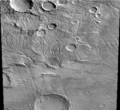
FIG. 1.: Viking Image for the Warrego Vallis (around $41^{\circ}$S, $91^{\circ}$W); some ”river-like”structures are present on the center-left (courtesy from NASA, PDS Planetary Image Atlas).

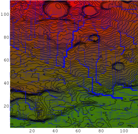
FIG. 2.: Computer reconstruction of the landscape in the area of Warrego Vallis; the main crater on the top left of Fig.1 is at the center of the red area.

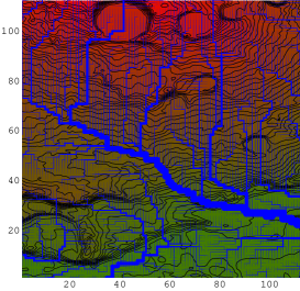
FIG. 3.: Computer reconstruction of the landscape in the area of Warrego Vallis, after pit removal. The reconstructed river structure is ”reasonably” similar to the visible one from Fig.1. Moreover it is evidently composed of patches of the channels in Fig.2

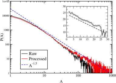
FIG. 4.: Histogram of the areas for the Warrego Vallis. Inset: the log-log plot of same histogram, binned over area intervals of ratio $1.5$; the dashed line has slope $0.5$.

REFERENCES

- [1] M.C. Malin and K.S. Edgett, Science 288, 2330 (2000).
- [2] M.C. Malinand K.S. Edgett, Science 290, 1927 (2000).
- [3] J.W. Head et al., Science 286, 2134 (1999).
- [4] P.D. Lanagan, A.S. McEwen, L.P. Keszthelyi and T. Thordarson, Geophys. Res. Lett. 28, 2365 (2001).
- [5] I. Rodriguez-Iturbe and A. Rinaldo Fractal Rivers Basins, Chance and Self-Organization Cambridge University Press, Cambridge (1997).
- [6] D.G. Tarboton, R.L. Bras and I. Rodriguez-Iturbe, Water Resour. Res. 24, 1317 (1988).
- [7] J.T. Hack, U.S. Geol. Survey Prof. Paper 294-B, 1 (1957).
- [8] L. Band Water Resour. Res., 22 15 (1986).
- [9] W.E. Dietrich, C.J. Wilson, D.R. Montgomery and J. McKean, J. Geol. 20, 675 (1992).
- [10] A. Maritan et al., Phys. Rev. E 53, 1510 (1996).
- [11] A. Coniglio, Phys. Rev. Lett. 62, 3054 (1989).
- [12] I. Rodriguez-Iturbe et al., Water Resour. Res. 28, 1095 (1992).
- [13] Z. Peizhen, P. Molnar and W.R. Downs, Nature 410, 891 (2001).