[

Kondo effect in Ce_xLa_1-xCu_2.05Si₂ intermetallics

Abstract

The magnetic susceptibility and susceptibility anisotropy of the quasi-binary alloy system Ce_xLa_1-xCu_2.05Si₂ have been studied for low concentration of Ce ions. The single-ion description is found to be valid for $x\leq 0.09$. The experimental results are discussed in terms of the degenerate Coqblin-Schrieffer model with a crystalline electric field splitting $\Delta\simeq 330$ K. The properties of the model, obtained by combining the lowest-order scaling and the perturbation theory, provide a satisfactory description of the experimental data down to 30 K. The experimental results between 20 K and 2 K are explained by the exact solution of the Kondo model for an effective doublet.

]

A Introduction

The intermetallic compound Ce_xLa_1-xCu_2.05Si₂ has been studied for more than two decades, but its properties are still not completely understood. For a large concentration of Ce ions the compound shows heavy fermion superconductivity [1] and small-moment antiferromagnetism. [2, 3] At intermediate concentrations, non-Fermi-liquid features are found, [4] while for small $x$ one observes anomalies due to the crystalline electric field splitting (CF) and the Kondo effect. [5, 6, 7] The change of the properties of the compound induced by Ce doping is an important issue that remains to be clarified, both experimentally and theoretically.

Here we present magnetic susceptibility data of Ce_xLa_1-xCu_2.05Si₂ intermetallics for small concentrations of Ce ions, $x\leq 0.09$, and show that the magnetic moment of Ce depends on temperature and is very anisotropic. [8] The samples we consider are sufficiently dilute for the interaction between the Ce ions to be neglected. We find the susceptibility of a single Ce ion embedded in a tetragonal host by studying the effects of Ce concentration. The magnetic anomalies are accompanied by transport anomalies, as indicated by large peaks in the thermoelectric power and a logarithmic increase of the electric resistance. [7] This behavior is typical of exchange scattering on CF-split ions and we base the theoretical analysis on the degenerate Coqblin-Schrieffer model [11] in which the two lowest CF states are coupled by exchange interaction to conduction states.

The CF parameters of dilute Ce alloys are obtained by analyzing the high-temperature magnetization data with the usual CF theory which neglects the coupling between the $f$ electrons and the conduction states, and considers just an isolated Ce ion in a tetragonal environment (for details see the Appendix). The magnetic anisotropy is explained by taking $\Delta\simeq 330$ K for the CF splitting between the doublet ground state and a pseudo quartet, formed by the two closely-spaced excited doublets, and taking $\eta=0.816$ for the relative weight of the CF orbitals. These values are consistent with the high-temperature neutron scattering data on CeCu₂Si₂ single crystals. [13, 14] However, the CF theory does not describe correctly the response of the high-temperature local moment, and it also fails to explain the rapid reduction of the local moment at intermediate temperatures and the loss of anisotropy at low temperatures. These characteristic features of the magnetic response of Ce ions in metallic hosts can only be obtained by coupling the $f$ states to the conduction band.

In this paper we show that the magnetic properties of dilute Ce_xLa_1-xCu_2.05Si₂ compounds can be explained by describing the interaction between the Ce ions and the metallic electrons by the Coqblin-Schrieffer model with the CF splitting. The high-temperature susceptibility obtained by the lowest-order perturbation theory agrees very well with the experimental data, provided we renormalize the exchange interaction by the ‘poor man’s scaling’.[15, 16, 17] For large CF splitting, the scaling theory generates two relevant low-energy scales, $T_{K}\ll T_{K}^{H}$, instead of one without splitting. The behavior of the anisotropic susceptibility above 30 K is accounted for by choosing $T_{K}=8.5$ K and $T_{K}^{H}=100$ K. The two low-energy scales, which differ by an order of magnitude, explain the reduction of the local moment from a high-temperature sextet to a low-temperature doublet, and lead to a qualitative explanation of the transport data.[7, 9] The low temperature properties of the Coqblin-Schrieffer model can not be calculated by scaling. However, for $\Delta=330$ K and $T_{K}^{H}=100$ K, the occupation of the excited CF states below 20 K is negligibly small. Thus, we approximate the $f$ state by an effective doublet, and describe the low-temperature properties by an effective spin-1/2 Kondo model with Kondo scale $T_{K}$. The exact renormalization group results for the susceptibility[18] agree very well with the experimental data.

The paper is organized as follows. First we describe the sample preparation and provide the details of the measurements. Then we analyze the susceptibility data obtained by the Faraday magnetometer on powdered samples and the anisotropy data obtained by the torque magnetometer on polycrystalline samples, and show that the observed anomalies can not be explained by the CF effects due to an isolated $f$ state. The coupling between the $f$ state and the conduction band, as described by the Coqblin-Schrieffer model with a CF splitting, is introduced next. Then, we discuss the susceptibility and the magnetic anisotropy of an excited quartet separated from the ground state doublet by the energy $\Delta$. Finally, compare the theoretical results the experimental data. The CF calculations for Ce ions in a tetragonal environment are presented in the Appendix.

B Experimental details and data analysis

1 The samples

The polycrystalline Ce_xLa_1-xCu_2.05Si₂ samples with low Ce-content $(x\leq 0.09)$ were prepared using a two-step procedure in order to enhance composition control and improve homogeneity. In the first step, appropriate amounts of pure elements were arc-melted to get master ingots with compositions $x=0$ and $x=0.1$. In the second step, part of these master ingots were melted together in an appropriate ratio to obtain samples with $0.01\leq x\leq 0.09$. Samples with larger Ce-content were prepared in a single step directly from pure elements. All samples were annealed for 40 hrs at 700 ^∘C, then for 80 hrs at 950 ^∘C, followed by a slow cooling to 700 ^∘C within 72 hrs. The X-ray powder diffraction patterns showed only reflections of the ThCr₂Si₂ structure. Both lattice parameters $a$ and $c$, as well as the unit cell volume, decrease linearly with increasing Ce content, the decrease being quite pronounced for $a$ but rather weak for $c$. [7] This preparation procedure combines all the experience gained in our laboratory within the last twenty years upon the investigation of CeCu₂Si₂ and related alloys. More detailed information about the preparation process can be obtained directly from the authors.[19]

The temperature dependence of the susceptibility $\chi(x,T)$ is found by measuring the fixed powders weighing about 20 mg. The data analysis shows that $\chi(x,T)$ is dominated by the contribution due to Ce ions, but that the samples with the same nominal Ce Concentration [20] show slightly different susceptibilities at low temperatures. This is demonstrated in Fig. 1, where $\chi(x,T)$ is plotted as a function of temperature for two pairs of typical samples. The susceptibility difference for the two samples with the same nominal concentration $x=0.07$ grows from about $2\times 10^{-6}$$(emu/mol)$ at 300 K to about $200\times 10^{-6}$$(emu/mol)$ at 2 K, while $\chi(x,T)$ increases in the same temperature interval only about 10 times. Similar behavior is seen in other samples, and we take that as an evidence that the susceptibility difference shown in Fig. 1 is not due to an inhomogeneous distribution of Ce ions. The slight variation of the functional form of $\chi(x,T)$ is most pronounced at low temperatures (see also Fig.5), and that can be explained in terms of a small variation in the Kondo temperature $T_{K}$. The inset in Fig. 1 shows the data for the two samples with nominally 7 at% of Ce, plotted versus $T/T_{K}$. The low–temperature data follow the same curve, provided we use $T_{K}=7.6$ K and $T_{K}=9.3$ K for the data represented by the open and filled triangles, respectively.[21] However, at intermediate temperatures, the data represented by the open and filled symbols can not be represented by a single function of $T/T_{K}$. The Kondo temperature of various samples might differ because of small deviations of the actual Cu concentration from the nominal one and the associated chemical pressure effects.

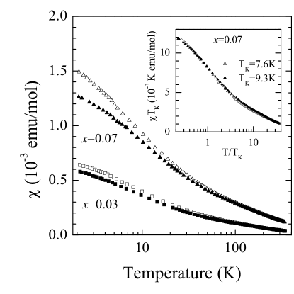
FIG. 1.: $\chi(x,T)$ plotted versus temperature for two pairs of Ce_xLa_1-xCu_2.05Si₂ samples. The triangles correspond to $x=0.07$ and the squares to $x=0.03$, respectively. The inset shows $\chi(x,T)\cdot T_{K}$ for the two $x=0.07$ samples, plotted versus $T/T_{K}$, with two different values of $T_{K}$.

The samples used for the torque measurements are small polycrystallites of irregular shape. The uniaxial symmetry of the unit cell allows one to obtain the intrinsic anisotropy even in the absence of perfect alignment of the crystallites (for details see below).

2 The susceptibility

The absolute value of the average magnetic susceptibility $\chi(x,T)$ is measured for Ce_xLa_1-xCu_2.05Si₂ samples on a high-precision Faraday balance for temperatures between 2 K and 350 K, for the magnetic field up to 9 kOe, and for Ce concentration ranging from 1 to 9 at%. The magnetization of all samples, measured at 300 K, 77 K, and 2 K, is found to be a linear function of the applied field. Susceptibility is defined as $\chi(x,T)=M/H$ $[emu/mol]$. The experimental results are plotted in Fig. 2 as a function of temperature and in Fig. 3 as a function of concentration. Fig. 3 shows that the susceptibility increase linearly with Ce concentration, and we take that as an evidence that the Ce-Ce interaction is small.

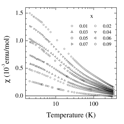
FIG. 2.: Susceptibility of Ce_xLa_1-xCu_2.05Si₂ plotted versus temperature on a logarithmic scale for $x\leq 0.09$.

The data analysis shows that the high–temperature susceptibility of the samples with the lowest concentration of Ce is diamagnetic, i.e., the response of very dilute alloys is dominated by a background. Thus, the effects of the alloying on the matrix in which the Ce ions fluctuate should not be a priory neglected. We also notice that the low–temperature susceptibility has a Curie-like upturn due to some unspecified magnetic impurities that are immanent to the rare earths, and for very dilute alloys this upturn becomes relatively large. Because the concentration of these unspecified magnetic impurities differs in each sample, and because the alloying changes the background, we do not define the single–ion Ce–response as a difference between the susceptibility of Ce_xLa_1-xCu_2.05Si₂ and LaCu_2.05Si₂. To minimize the systematic error due to sample preparation we define the susceptibility of a Ce–free compound as a statistical average obtained from Fig. 3, and find the single–ion contribution by the following procedure.

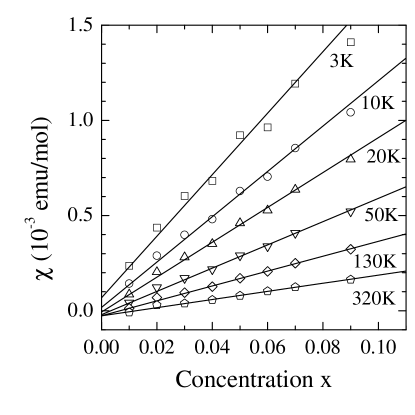
FIG. 3.: Susceptibility of Ce_xLa_1-xCu_2.05Si₂ plotted versus concentration for various temperatures.

We assume that the total susceptibility of a given sample, which is shown in Figs. 2 and  3, comprises two contributions: a single-ion Ce susceptibility, $\chi_{ion}$, and a concentration-dependent background, $\chi_{B}(x,T)\simeq\chi(0,T)+x\cdot\left[\partial\chi_{B}(x)/\partial x\right]_{x=0}.$ We consider only the lowest order concentration effects and express the measured susceptibility of a given sample as,

$$\chi(x,T)=\chi(0,T)+x\left\{\chi_{ion}(T)+\left[\partial\chi_{B}(x)/\partial x\right]_{x=0}\right\}.$$ (1)

To find $\chi_{B}(x,T)$ we notice that the susceptibility data shown in Fig. 3 are linear in concentration for all temperatures, and use the $x=0$ intercept of the straight lines to define the statistically averaged background susceptibility of the Ce-free matrix, $\chi(0,T)$. The values obtained in such a way are shown in Fig. 4, together with the least-squares fit based on the expression

$$\chi(0,T)=\chi_{0}+\frac{C_{imp}}{T-\Theta_{imp}},$$ (2)

where $\chi_{0}$ describes the constant diamagnetic contribution of the stoichiometric compound LaCu_2.05Si₂ and the Curie-Weiss term describes magnetic contamination. The experiment gives, $\chi_{0}=-3.1\cdot 10^{-5}$ $(emu/mol)$, $C_{imp}=5.9\cdot 10^{-4}\;$K ($emu/mol$), and $\Theta_{imp}=-2.8$ K. To estimate the level of contamination we assume $C_{imp}=(N_{imp}/3k_{B})g^{2}\mu_{B}^{2}j(j+1)$, where $\mu_{B}$ is Bohr magneton, $g$ is the gyromagnetic factor and $k_{B}$ is Boltzmann constant. Taking for $j$ the smallest possible value, $j=1/2$, we find that the upper limit for the number of magnetic impurity atoms is $N_{imp}=0.0016\;N_{A}$, where $N_{A}$ is Avogadro number. Thus, the average concentration of the unspecified magnetic impurities is about $0.1$ at%, which is at least one order of magnitude less than the lowest Ce concentration we measure.

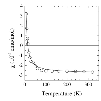
FIG. 4.: The susceptibility of the LaCu_2.05Si₂ matrix $\chi(0,T)$ plotted versus temperature (circles). The full line is the least-squares fit by Eq. (2). The low-temperature Curie-Weiss upturn is due to magnetic contamination. Note the difference in the vertical scales used here and in Fig. 2.

Using Eqs. (1) and (2) we find that $[\chi(x,T)-\chi(0,T)]/x$ defines the same curve for all the samples. This unique curve defines the impurity susceptibility $\chi_{ion}(T)$ up to a constant shift $\left[\partial\chi_{B}(x)/\partial x\right]_{x=0}$. However, the two terms in the braces in Eq. (1) can not be obtained by independent measurements, and we replace $\chi_{ion}(T)$ in Eq. (1) with a theoretical expression (for details see below) and find that the experimental data can be fitted by taking $\left[\partial\chi_{B}/\partial x\right]_{x=0}=10^{-4}$($emu/mol$ Ce). The same value of this constant shift is obtained by using for the high-temperature single-ion susceptibility in Eq. (1) the expression $\chi_{ion}(T)\sim 1/T$, and making the least-squares fit through the data above 250 K. The comparison of $\chi_{ion}(T)$ and $\partial\chi_{B}(x)/\partial x$ shows that the susceptibility contribution due to Ce ions is at least one order of magnitude larger than the background contribution, so that a possible small error in $\left[\partial\chi_{B}(x)/\partial x\right]_{x=0}$ does not influence our conclusions in an essential way.

The average susceptibility of a single Ce ion in dilute Ce_xLa_1-xCu_2.05Si₂ samples is defined by the expression

$$\chi_{ion}(T)=\frac{\chi(x,T)-\chi(0,T)}{x}-10^{-4}(emu/mol\;Ce),$$ (3)

which is shown in Fig.5 as a function of temperature for various values of $x$. The response of Ce ions is nearly the same for all the compounds up to $x\simeq 0.09$, and it begins to deviate from the $x$-independent form for $x\geq 0.1$.[8] The scatter of the data at low temperatures is about the same as the scatter shown in Fig. 1, and can be eliminated by plotting $\chi_{ion}$ on a universal temperature scale $T/T_{K}(x)$, with $T_{K}(x)=8.5\pm 1$ K. However, in our dilute samples, the lack of any systematic behavior of $T_{K}(x)$ as a function of Ce–doping does not allow us to explain the observed fluctuations in terms of the chemical pressure effects induced by Ce doping. As discussed in the previous section, the random variation of $T_{K}(x)$ can be associated with the local fluctuations in Cu stoichiometry.

The anomalous behavior of the molar susceptibility of Ce in Ce_xLa_1-xCu_2.05Si₂ becomes most transparent if one compares $\chi_{ion}(T)$ with the susceptibility of a crystalographically equivalent but unhybridized $4f^{1}$ state, $\chi_{CF}(T)$, which is calculated in the Appendix. In Fig.5 we plot the susceptibilities versus $\log T$, and in Fig.6 we use the Curie-Weiss plot and show the inverse of the susceptibilities as a function of $T$. The symbols represent the experimental data, while the dashed line, the full line and the dashed-dotted line represent the CF, the scaling, and the Wilson’s result, respectively.

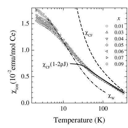
FIG. 5.: The average single-ion susceptibility of Ce_xLa_1-xCu_2.05Si₂ defined as $\chi_{ion}(T)=[\chi(x,T)-\chi(0,T)]/x-1\cdot 10^{-4}$($emu/mol$ Ce), plotted versus temperature for $x\leq 0.09$ samples. The full line shows the scaling result, the dashed line shows the CF result and the dashed-dotted line shows the exact solution for the spin-1/2 Kondo model in the local moment regime.

The high-temperature susceptibility follows the Curie-Weiss law, $1/\chi_{ion}(T)\simeq(T-\Theta)/C$, where $C=N_{A}\mu_{\mathrm{e}ff}^{2}/3k_{B}\simeq 0.125\mu_{\mathrm{e}ff}^{2}/\mu_{B}^{2}\simeq 0.8$ K $emu/mol$ Ce, which is close to the CF result. The antiferromagnetic Weiss temperature is $\Theta\simeq-100$ K. The low-temperature susceptibility data can also be represented by a Curie-Weiss law with $C=0.3$ K $emu/mol$ Ce and $\Theta\simeq-15$ K. This value of $C$ leads to $\mu_{\mathrm{e}ff}\simeq 1.6\mu_{B}$ which is close to the average value obtained for the lowest CF doublet (see the Appendix).

The analysis of the single-impurity data in Figs. 5 and 6 shows clearly that the CF theory, which neglects the coupling of $f$ electrons to conduction states, fails to explain the response of the $4f^{1}$ ions to an external magnetic field. The correct description is obtained by considering not only the thermodynamic fluctuations but taking also into account the quantum fluctuations, due to Kondo effect. Before evaluating these effects in more detail, we discuss the torque measurements which provide the magnetic anisotropy of Ce ions and allow us to obtain the full susceptibility tensor.

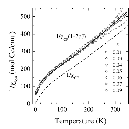
FIG. 6.: The inverse of the average single-ion susceptibility shown as a function of temperature for Ce_xLa_1-xCu_2.05Si₂ samples with $x\leq 0.09$. Dashed line is the CF result, and the full line is the scaling result.

3 The susceptibility anisotropy

The intrinsic anisotropy of polycrystalline Ce_xLa_1-xCu_2.05Si₂ samples with clear preferential orientation was measured on a high-precision torque magnetometer. In the experiment the sample is attached to a thin vertical quartz fiber and a homogeneous magnetic field ${\bf H}$ is applied in the horizontal $xy$ plane, as shown in Fig. 7. Thus, only the $z$ component of the torque ${\bf\Gamma}$ is measured.

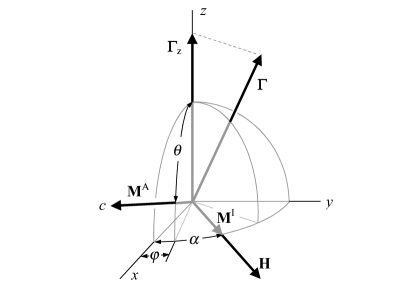
FIG. 7.: The torque on a uniaxial crystallite, oriented along $c$ direction, induced by the external magnetic field H in the $xy$ plane.

The experimental values for the susceptibility anisotropy of a given sample $\Delta\chi^{exp}$ are obtained from the ratio $\Gamma_{z}/H^{2}$, which is measured by the following procedure. For an arbitrary sample orientation, the magnetic field is rotated in the $xy$ plane by an angle $\alpha$ varying from 0⁰ to 180⁰. Measuring the angular dependence of the torque curve at 300 K, 77 K and 2 K, in a magnetic field of 8 kOe, we find that $\Gamma_{z}(\alpha)$ is a sinusoidal function of a period $\pi$, with zeros which are independent of temperature. This shows that the magnetization of the sample is proportional to the applied field. The amplitude $\Gamma^{(h)}_{z}$ of the sine torque curve is then measured as a function of temperature. Next, the sample is rotated by 90⁰ around the $y$ axis, and the amplitude $\Gamma^{(v)}_{z}$ is measured as a function of temperature. The experimental anisotropy of a given sample is defined as $\Delta\chi^{exp}_{i}=2\Gamma_{z}^{(i)}/H^{2}n$ $[emu/mol]$, where $n$ is the number of moles and the index $i=h,v$ denotes the two orientations of the sample. The data obtained in this way are shown in Fig. 8 where $\Delta\chi^{exp}_{i}(x,T)$ is plotted versus temperature for $x=0.01,0.02,0.03$, and $0.06$. All of the curves in Fig. 8 show similar temperature dependence, with the extremum point at 48 K. The torque signal is quite strong due to a large anisotropy of the Ce moment and because the measurements are performed on samples with a rather high degree of preferential alignment of the crystallites within the polycrystal.

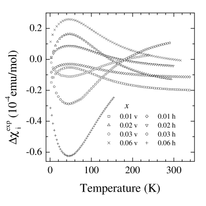
FIG. 8.: The susceptibility anisotropy of Ce_xLa_1-xCu_2.05Si₂ is shown as a function of temperature for $x\leq 0.06$ samples. The data corresponding to two different orientations of the sample with respect to the magnetic field are denoted by $h$ and $v$, respectively.

To analyze the torque data shown in Fig. 8 we write the $z$ component of ${\bf\Gamma}$ as

$$\Gamma_{z}=V({\bf M}\times{\bf H})_{z},$$ (4)

where $V$ is the volume of the sample and M is the magnetization induced by H. For a single tetragonal crystallite, the induced magnetization has an isotropic and an anisotropic component, i.e., it can be written as

$${\bf M}={\bf M}^{I}+{\bf M}^{A},$$ (5)

where the isotropic component M^I is directed along H, while the anisotropic one M^A is directed along the $c$ axis of the crystal. Obviously, ${\bf M}^{I}=\chi^{ab}{\bf H}$ and ${\bf M}^{A}=(\chi^{c}-\chi^{ab}){\bf H}_{c}$, where $\chi^{c}$ is the susceptibility along the $c$ axis, $\chi^{ab}$ is the susceptibility in the $ab$ plane, and ${\bf H}_{c}$ is the component of the magnetic field along the $c$ direction. Using Eq.(4), we find that the torque on a crystallite with the $c$ axis directed along $(\theta,\varphi)$, and induced by the magnetic field in the $xy$ plane, ${\bf H}=H(\cos\alpha,\sin\alpha,0)$, is given by the expression (see also Fig. 7)

$$\Gamma_{z}=\frac{1}{2}nH^{2}\Delta\chi\sin^{2}(\theta)\sin\left[2(\alpha-\varphi)\right],$$ (6)

where $\Delta\chi$ is now measured in $emu/mol$, i.e., stands for $(V/n)\Delta\chi$. Thus, the temperature dependence of the torque is given, up to a numerical constant, by the intrinsic susceptibility anisotropy $\Delta\chi=\chi^{c}-\chi^{ab}$, regardless of the orientation of the crystallite.

In a polycrystalline sample, we are dealing with some volume distribution $V_{i}=V_{i}(\theta_{i},\varphi_{i})$ of the crystallites with respect to their orientations. The total torque on a sample with a given concentration of Ce ions is the sum of all the separate contributions and can be written as

$$\Gamma^{x}_{z}=\frac{1}{2}nH^{2}\gamma_{x}\Delta\chi\sin\left[2(\alpha-\bar{\varphi}_{x})\right],$$ (7)

where we introduced the alignment factor $\gamma_{x}$ $(0\leq\gamma_{x}\leq 1)$ and the phase shift $\bar{\varphi}_{x}$. In our experiment the magnet is rotated to a position $\alpha-\bar{\varphi}_{x}=\pm\pi/4$ which maximizes the torque. Thus, up to a geometrical factor $\gamma_{x}$, the temperature dependence of the torque follows from the intrinsic anisotropy of the sample. The alignment factor $\gamma_{x}$ depends on the distribution of the polycrystallites in the sample, and is given by $\gamma_{x}=\sqrt{A_{x}^{2}+B_{x}^{2}}$, where $A_{x}=\frac{1}{V}\sum_{i}V_{i}\sin^{2}\theta_{i}\cos 2\varphi_{i}$ and $B_{x}=\frac{1}{V}\sum_{i}V_{i}\sin^{2}\theta_{i}\sin 2\varphi_{i}$. To find the single-ion anisotropy we have to estimate $\gamma_{x}$ and the intrinsic anisotropy of the metallic matrix.

The data analysis shows that the experimental anisotropy $\Delta\chi^{exp}(x,T)=\gamma_{x}\Delta\chi$ follows a similar temperature dependence in all the samples. This is shown in Fig. 9, where $\Delta\chi_{i}^{exp}(x,T)$ is plotted as a function of $\Delta\chi_{v}^{exp}(x_{1},T)$, with temperature as an implicit variable. We recall that index $i=v,h$ denotes the orientation of the sample with respect to the applied field. The orientation of the reference sample is $v$ and the referent Ce concentration is $x_{1}=0.01$. The correlation between the torque data is found to be strictly linear,

$$\Delta\chi_{i}^{exp}(x,T)=k_{x}^{i}\Delta\chi^{exp}_{v}(x_{1},T)+l_{x}^{i},$$ (8)

where $k_{x}^{i}$ and $l_{x}^{i}$ denote the slope and the intercept of the straight lines respectively. The numerical values of $k_{x}^{i}$ and $l_{x}^{i}$ for each sample are given in Table I. As shown below, the linear relation (8) proves essential for obtaining the single-ion contribution from the experimental anisotropy data.

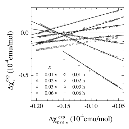
FIG. 9.: $\Delta\chi_{i}^{exp}(x,T)$ of Ce_xLa_1-xCu_2.05Si₂ samples is plotted versus $\Delta\chi_{v}^{exp}(x_{1},T)$. The data are given for two different orientations ($i=h,v$) with respect to H. The concentration of the Ce ions in the referent sample is $x_{1}=0.01$. The full lines are the linear extrapolations which define the coefficients $k_{x}^{i}$ and $l_{x}^{i}$.

In analogy with the analysis of the susceptibility data we assume that the susceptibility anisotropy of a given crystallite has a single-ion contribution, $\Delta\chi_{ion}(T)=\chi_{ion}^{c}-\chi_{ion}^{ab}$, and a van Vleck contribution due to the matrix, $\Delta\chi_{B}=\chi_{B}^{c}-\chi_{B}^{ab}$. The unspecified magnetic impurities which contaminate our samples, and which are described by Eq. (2), are assumed to be isotropic, because the the torque shown in Fig. 8 has no Curie-like upturn. Thus, we write the susceptibility anisotropy of a given sample as

$$\Delta\chi_{i}^{exp}(x,T)=\gamma_{x}^{i}\left[x\,\Delta\chi_{ion}(T)+\Delta\chi_{B}(x)\right],$$ (9)

where the temperature dependence of $\Delta\chi_{B}$ is neglected. In the dilute limit, we approximate the van Vleck anisotropy by a linear expression $\Delta\chi_{B}(x)\simeq\Delta\chi_{0}+x\left[\frac{\partial\Delta\chi_{B}(x)}{\partial x}\right]_{x=0}$, and use Eqs. (8) and (9) to derive an approximate relation between the experimentally determined quantities

$$\frac{l_{x}^{i}x}{k_{x}^{i}(x-x_{1})}=-\gamma^{v}_{1}\Delta\chi_{0},$$ (10)

where $\gamma^{v}_{1}$ is the alignement factor of the referent sample. The experimental values obtained from Fig. 9 indicate that the ratio in Eq. (10) is indeed very nearly sample-independent, and given by $\gamma^{v}_{1}\Delta\chi_{0}\simeq-2.4\cdot 10^{-5}$$[emu/mol]$. Using this value, and Eqs. (8) and (9), we can express the product ${\gamma^{v}_{1}}\Delta\,\chi_{ion}(T)$ in terms of experimentally determined quantities, [22]

$${\gamma_{1}^{v}}\Delta\,\chi_{ion}(T)=\left[\frac{\Delta\chi_{i}^{exp}(x,T)-l_{x}^{i}}{x_{1}k_{x}^{i}}-\frac{\gamma^{v}_{1}\Delta\chi_{0}}{x_{1}}\right].$$ (11)

Considering ${\gamma^{v}_{1}}\Delta\,\chi_{ion}(T)$ as a function of temperature one obtains the same function for all the samples. The value of $\gamma^{v}_{1}$ is obtained by fitting the universal curve (11) by the theoretical result for the Coqblin-Schrieffer model, with the same parameters as in the previous section. This gives $\gamma^{v}_{1}=0.55$.

FIG. 10.: The single-ion susceptibility anisotropy $\Delta\chi_{ion}(T)$ defined by Eq. (11) plotted versus temperature for all the Ce_xLa_1-xCu_2.05Si₂ samples with $x\leq 0.06$. The full line is the scaling result, and the dashed line is the CF result.

The single-ion anisotropy $\Delta\chi_{ion}(T)$, defined in the above described way, is plotted as a function of temperature in Fig. 10, together with the scaling result (full line) and the CF anisotropy (dashed line). The data show clearly that the magnetic anisotropy of $4f^{1}$ ions in the tetragonal Ce_xLa_1-xCu_2.05Si₂ crystals can not be explained by the CF theory, which considers only the thermal fluctuations among various CF states. The correct description is obtained by including the quantum fluctuations, and is provided here by the scaling solution of the Coqblin-Schrieffer model.

C Theoretical analysis

The properties of Ce ions in dilute Ce_xLa_1-xCu_2.05Si₂ samples are modeled by the Coqblin-Schrieffer Hamiltonian with CF splitting,

$$H_{K}=H_{CF}+H_{0}+H_{J},$$ (12)

where $H_{CF}$ describes the $f$ states in the tetragonal CF (see the Appendix), $H_{0}$ describes the conduction band of width $2D_{0}$, with a constant density of states $\rho$, and $H_{J}$ defines the exchange coupling between the $4f^{1}$ states and the band electrons. [11, 12]

The high-temperature properties are calculated by the poor man’s scaling, [15, 16, 17] which provides the renormalized coupling by reducing the conduction electron cutoff from $D_{0}$ to $D$, and simultaneously rescaling the coupling constant from $J_{0}$ to $J(D)$, so as to keep the low-energy excitations of the total system unchanged. Assuming the isotropic exchange, this leads to [16, 17]

$$\rho J\exp\left(-\frac{1}{\rho J}\right)=\left(\frac{k_{B}T_{K}}{D}\right)^{m}\left(\frac{k_{B}T_{K}+\Delta}{D+\Delta}\right)^{M},$$ (13)

where $J$ is the absolute value of the antiferromagnetic coupling constant, $m=2$ and $M=4$ are the degeneracies of the lower and the upper CF state, respectively, $\Delta$ is the CF splitting, and $T_{K}$ is the Kondo temperature. The renormalized coupling constant $J(D)$ defines an effective model with cutoff $D$. The Kondo temperature is given by Eq. (13) with $J$ and $D$ replaced by the initial values $J_{0}$ and $D_{0}$, respectively (for details see [16, 17]). The scaling law (13) applies provided the renormalized coupling is small, i.e., $\rho J\ll 1$ and $D\gg T_{K}$.

The scaling trajectory described by Eq.(13) has two asymptotic regimes. The high-temperature asymptote, $J_{H}(T)$, is obtained by neglecting the CF splitting, and is given by,

$$\rho J_{H}\exp\left(-\frac{1}{\rho J_{H}}\right)=\left(\frac{k_{B}T^{H}_{K}}{D}\right)^{N},$$ (14)

where, $T^{H}_{K}$ is the high-temperature Kondo scale, defined by Eq.(14) with $J_{0}$ and $D_{0}$ replacing $J_{H}$ and $D$, respectively.

The low-temperature asymptote $J_{L}(D)$ is obtained by neglecting in Eq.(13) the effects of the excited CF levels, i.e., by neglecting $T_{K}$ and $D$ with respect to $\Delta$. This identifies $J_{L}(D)$ as the scaling trajectory of an effective doublet with Kondo scale $T_{K}$, and the effective coupling,

$$\rho J_{L}\exp\left(-\frac{1}{\rho J_{L}}\right)=\left(\frac{k_{B}T_{K}}{D}\right)^{m}.$$ (15)

Eqs.(13 - 15), show that the $f$ level behaves at high temperatures as an effective sextet with Kondo scale $T_{K}^{H}$, and at low temperatures as an effective doublet with Kondo resonance $T_{K}$. The two Kondo scales satisfy the relation,

$$(k_{B}T_{K}^{H})^{m+M}=(k_{B}T_{K})^{m}\Delta^{M}.$$ (16)

The scaling result given by Eq.(13) shows that we can remove the CF splitting from the asymptotic considerations at high and low temperatures, provided we renormalize the effective coupling constant in such a way that the low-energy properties of the effective models and the Coqblin-Schrieffer model are the same. Note, the $T_{K}$ of the effective doublet is much higher than the Kondo scale of the Coqblin-Schrieffer model calculated in the limit $\Delta\gg D_{0}$, with the initial condition $J_{L}(D_{0})=J_{0}$.

The anisotropic susceptibility tensor of the Coqblin-Scrieffer model with CF splitting is obtained by applying the linear response theory, and calculating the response functions by lowest-order perturbation theory with renormalized coupling constants[23, 24, 25, 26]. The effective Coqblin-Schrieffer model at a given temperature T is obtained by reducing the cutoff from $D_{0}$ to $D=A\,k_{B}T$, and renormalizing $J_{0}$ to $J(T)=J(T_{K}/AT,\Delta/Ak_{B}T)$ according to Eq. (13). Here, A is a numerical constant of the order of unity. Thus, we obtain the susceptibility

$$\chi^{\alpha}_{J}(T)=\chi_{CF}^{\alpha}(T)[1-2\rho J(T)],$$ (17)

where $\chi_{CF}^{\alpha}(T)$ is the $\alpha$ component of the anisotropic CF susceptibility calculated in the Appendix. The result  (17) shows that the exchange interaction reduces the CF susceptibility, and the poor man’s scaling gives the reduction factor as $F(T,T_{K},\Delta)=[1-2\rho J(T)]$. Fitting the experimental results above 30 K with the renormalized susceptibility given by Eq.(17), where $J(T)$ is given by Eq.(13), we obtain an implicit relation between $T_{K}$ and the cutoff constant A. The analysis of the Ce_xLa_1-xCu_2.05Si₂ data above 30 K shows that we van write $T_{K}\simeq\alpha A+\beta$, where $\alpha=3$ K and $\beta=-1$ K. The physically acceptable range of the cutoffs is from $k_{B}T$ to $4k_{B}T$, which gives $T_{K}$ between 2 K and 11 K, and $T_{K}^{H}$ between 60 and 110 K. However, the analysis of the low–temperature data (see below) leads to the values $T_{K}=8.5$ and $A=3$. The theoretical results obtained in such a way are shown in Figs. 5, 6, 10, 11, and 12 as a full line.

The experimental data are described by the scaling theory down to 30 K. At lower temperatures there is a discrepancy, which is not really surprising, since $J(T)$ in Eq.(17) grows rapidly for $T\ll T_{K}^{H}$ and at about 30 K the coupling given by Eq.(13) becomes too large for the renormalized perturbation expansion to be valid. Note, in the absence of the CF splitting the perturbation theory for the $N$-fold degenerate $f$ level breaks down at around $T\simeq T_{K}^{H}$. The CF splitting reduces the degeneracy of the ground state and extends the validity of the perturbation expansion down to about $T\simeq AT_{K}$, where $T_{K}$ is the Kondo temperature of the effective doublet, and $T_{K}\ll T_{K}^{H}$.

Below 20 K, however, the coupling constants defined by Eqs.(13) and (15) satisfy $J(T)\simeq J_{L}(T)$, such that we can consider the $f$ state as an effective doublet. The average moment of the CF ground state, calculated by the CF theory, is $\mu=1.62\mu_{B}$, which is not too different from the free spin-1/2 moment, $\sqrt{3}\mu_{B}$. Thus, to discuss the low-temperature data, for $T\leq T_{K}$ we neglect the small anisotropy of the CF ground state and approximate the CF split multiplet by an effective doublet, and replace the Coqblin-Schrieffer model by an effective spin-1/2 Kondo model. We relate the two models by setting the Kondo temperature of the spin-1/2 Kondo problem to $T_{K}$. In such way the parameter space of the low–temeperature model is completly determined. The susceptibility of the Kondo model in the local moment (LM) regime, i.e., for $T_{K}/2\leq T\leq 15T_{K}$, is given by the numerical renormalization group result[18]

$$\chi_{W}=\frac{0.68C_{0}}{T+\sqrt{2}T_{K}},$$ (18)

where $C_{0}={N_{A}(g\mu_{B})^{2}S(S+1)}/{3k_{B}}$, i.e., $C_{0}=0.375$ $emu/mol$. Using $\chi_{W}$ and $T_{K}=8.5$ K we obtain the curve shown in Figs. 5 and 12. In the low-temperature LM regime, which sets in for diluite Ce_xLa_1-xCu_2.05Si₂ alloys between 4 K and 30 K, we find that the calculated susceptibility is very close to the experimental values. Thus, by demanding that the low– and the high–temperature models have the same Kondo temperature we restricted the high–temperature cutoff constant to $A=3$.

D Discussion of the experimental results and conclusion

The anisotropic susceptibility of a single Ce ion is found by systematic measurements of dilute Ce_xLa_1-xCu_2.05Si₂ alloys on the Faraday balance and the torque magnetometer, and by carefully subtracting the background. The experimental results are explained by the Coqblin-Schrieffer model with the CF doublet-quartet splitting $\Delta=330$ K and with the exchange scattering such that $T_{K}=8.5\,$K. The average value of the calculated susceptibility tensor, $\chi_{J}(T)=[2\chi^{ab}_{J}(T)+\chi^{c}_{J}(T)]/3$, is shown in Figs. 5 and 6, together with the experimental data. The corresponding result for the susceptibility anisotropy $\Delta\chi_{J}(T)$ is compared with the torque measurements in Fig. 10. Combining the Faraday balance and the torque data we find the single-impurity response along the principal axes, which is shown in Fig.11 for the $x=0.06$ sample, together with the scaling result (full lines) and the CF theory (dashed lines). The experimental data for other samples are about the same.

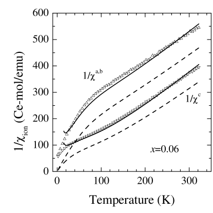
FIG. 11.: The single-ion susceptibility for finite Ce concentration shown on a Curie-Weiss plot as a function of temperature for Ce_0.06La_0.94Cu_2.05Si₂. Dashed line is the CF result $1/\chi^{\alpha}_{CF}(T)$, and full line is the scaling result $1/\chi^{\alpha}_{J}(T)$. The calculations are performed using $T_{K}=8.5$ K, $T_{K}^{H}=100$ K, and $\Delta=330$ K.

The principal-axes susceptibilities shown in Fig. 11 follow between 100 K and 350 K an anisotropic Curie-Weiss law,

$$\chi^{\alpha}_{ion}=\frac{C^{\alpha}}{T-\Theta^{\alpha}},$$ (19)

such that the slope of $1/\chi^{\alpha}_{ion}(T)$ and $1/\chi^{\alpha}_{CF}(T)$ is about the same. Thus, the high-temperature data can be discussed in terms of an anisotropic local moment which is close to the CF value. However, the response of the $f$ state is reduced with respect to the CF value due to the temperature dependent exchange coupling to the conduction band. The lowest order perturbation theory gives the reduction factor as $F(T/T_{K}^{H})=1-2\rho J_{H}(T/T_{K}^{H})$, where we assumed an isotropic exchange coupling. The Ce impurity behaves in this high-temperature LM regime as a sextet split by the tetragonal CF, and with the relevant Kondo scale $T_{K}^{H}=100$ K.

Below $T\simeq T_{K}^{H}$, we observe the crossover from the high-temperature LM regime to an effective twofold degenerate low-temperature LM regime. Surprisingly, the behavior of the system at the crossover is still rather well described by scaling, and the single-ion response can be discussed in terms of the reduced CF susceptibility.

At low temperatures, $T\leq A\ T_{K}$, the renormalized coupling becomes too large for the lowest-order renormalized perturbation expansion to be valid. Since we are not aware of any accurate theoretical results for the response of Coqblin-Schrieffer model with CF splitting that we can use close to $T_{K}$, we estimate the reduction factor $F(T)$ directly from the experiments, assuming that the exchange is isotropic and that the susceptibility retains the factorized form (17) down to lowest temperatures. The Faraday balance data give $F(T)=\chi_{ion}(T)/\chi_{CF}(T)$ and the torque data give $F(T)=\Delta\chi_{ion}(T)/\Delta\chi_{CF}(T)$, which we plot in Fig.12, together with the high-temperature scaling result $\chi_{J}/\chi_{CF}=[1-2\rho J(T)]$ and the Wilson’s result $F_{W}=T\chi_{W}/C_{0}$.

FIG. 12.: Temperature dependence of the reduction factor of the susceptibility, $F(T)=\chi_{ion}(T)/\chi_{CF}(T)$ for Ce_xLa_1-xCu_2.05Si₂ with $x\leq 0.09$. The symbols are obtained from the susceptibility data, the dashed line is obtained from the anisotropy data and the solid line is the scaling result. The dashed-dotted line shows the reduction factor for the spin-1/2 Kondo model.

The reduction factors obtained from the average susceptibility and the anisotropy data are very similar, and the high–temperature data are rather well described by the poor man’s scaling. At low temperatures, where the crystal field calculations lead to an effective doublet with $\chi_{CF}\simeq N_{A}\mu_{\mathrm{e}ff}^{2}/3k_{B}T$ and $\mu_{\mathrm{e}ff}\simeq 1.621\mu_{B}$, the experimental reduction factor comes very close to the universal curve obtained for the isotropic spin-1/2 Kondo model.[18]

We mention, for completeness, that the magnetic anomalies discussed here are accompanied by the usual Kondo anomalies in the electric resistivity and the thermoelectric power data. [7] All the samples used for the susceptibility measurements have a clear Kondo minimum in the bare resistivity, as well as a very large thermoelectric power with two peaks, which is typical of CF split Kondo ions.[27] The low-temperature peak is at about 10 K, and the high temperature one at about 120 K, as expected in a system described by the Coqblin-Schrieffer model with the Kondo scales, $T_{K}\simeq 8.5$ K and $T_{K}^{H}\simeq 100$ K.

In summary, the magnetic susceptibility of a dilute Ce ions embedded in the tetragonal metallic host has been obtained by careful data analysis. The samples used in our studies have a negligibly small Ce–Ce interaction. The changes in the matrix induced by the doping are also found to be very small. The behavior of the Ce_xLa_1-xCu_2.05Si₂ compounds with less than 9 at% of Ce is well described by the Coqblin-Schrieffer model of a $f$ state comprising a ground state doublet and a pseudoquartet split by $\Delta\simeq 330$ K. The quantum fluctuations due to the exchange coupling between the $f$ state and the conduction band can be described by the poor man’s scaling, which explains the high-temperature data and the crossover from the high-temperature LM regime to a twofold degenerate low-temperature LM regime, that takes place at about $T^{H}_{K}\simeq 100$ K. The lowest-order perturbation expansion, based on the scaling solution of the CF split model, breaks down below 30 K. However, at such low temperatures, the effect of the excited CF states is rather small, and the experimental results below 20 K can be described by the exact solution of the spin-1/2 Kondo model with Kondo scale $T_{K}=8.5$ K. This low–temperature Kondo scale determines completly the cutoff constant used in the high–temperature scaling.

E Acknowledgments

We acknowledge the useful comments from B. Horvatić. The financial support from the Alexander von Humboldt Foundation to VZ is gratefully acknowledged.

F Appendix

A Ce³⁺ ion in a tetragonal crystal field is described by the Hamiltonian[28]

$$H_{CF}=B_{2}^{0}O_{2}^{0}+B_{4}^{0}O_{4}^{0}+B_{4}^{4}O_{4}^{4},$$ (20)

where $B_{l}^{m}$ are the CF parameters and $O_{l}^{m}$ are the Stevens operators, which are related to the angular momentum operator $J$ and its components $J_{x}=\frac{1}{2}(J_{+}+J_{-})$, $J_{y}=\frac{1}{2i}(J_{+}-J_{-})$, and $J_{z}$, as follows:

$$O_{2}^{0}=3J_{z}^{2}-J(J+I),$$ (21)

$\displaystyle O_{4}^{0}=35J_{z}^{2}-30J(J+I)J_{z}^{2}+25J_{z}^{2}-6J(J+I)+3J^{2}(J+I)^{2},$

$\displaystyle O_{4}^{4}=\frac{1}{2}(J_{+}^{4}+J_{-}^{4}).$

For small CF this Hamiltonian is a perturbation to the sixfold degenerate $4f^{1},$ $j=5/2$ atomic wave functions $\left|\pm\frac{1}{2}\right\rangle,\left|\pm\frac{3}{2}\right\rangle,\left|\pm\frac{5}{2}\right\rangle,$ and it is easily diagonalized. The eigenvectors $\left|n\right\rangle$ are given by

$$\Gamma_{7}^{(1)} : \left|\pm 1\right\rangle=\eta\left|\pm\frac{5}{2}\right\rangle+\sqrt{1-\eta^{2}}\left|\mp\frac{3}{2}\right\rangle,$$ (22)

$$\hskip 36.135pt\Gamma_{7}^{(2)} : \left|\pm 2\right\rangle=-\sqrt{1-\eta^{2}}\left|\pm\frac{5}{2}\right\rangle+\eta\left|\mp\frac{3}{2}\right\rangle,$$ (23)

$$\Gamma_{6} : \left|\pm 3\right\rangle=\left|\pm\frac{1}{2}\right\rangle,$$ (24)

and the energy eigenvalues $\epsilon_{n}$ are

$$\epsilon_{1} = 10B_{2}^{0}+60B_{4}^{0}+12\sqrt{5}\frac{\sqrt{1-\eta^{2}}}{\eta}B_{4}^{4},$$ (25)

$$\epsilon_{2} = -2B_{2}^{0}-180B_{4}^{0}-12\sqrt{5}\frac{\sqrt{1-\eta^{2}}}{\eta}B_{4}^{4},$$ (26)

$$\epsilon_{3} = -8B_{2}^{0}+120B_{4}^{0},$$ (27)

where the mixing parameter $\eta$ is defined by the equation

$$\frac{\eta}{\sqrt{1-\eta^{2}}}-\frac{\sqrt{1-\eta^{2}}}{\eta}=\frac{B_{2}^{0}+20B_{4}^{0}}{\sqrt{5}B_{4}^{4}}.$$ (28)

The neutron scattering data[14] indicate a $\Gamma_{7}$ ground state and a CF scheme shown in Fig. 13.

FIG. 13.: The CF level for the doublet-quartet scheme used in the calculations.

Since $\epsilon_{2}\approx\epsilon_{3}$, we use here an approximate doublet-quartet scheme.

The $\alpha$ component of the CF susceptibility of one mole of isolated $Ce^{3+}$ ions is given by the van Vleck formula [29]

$$\chi_{CF}^{\alpha} = \frac{N_{A}(g_{J}\mu_{B})^{2}}{Z}\mathop{\displaystyle\sum}\limits_{n}\left[\beta\sum_{m,\epsilon_{n}=\epsilon_{m}}\left|\langle m\mid J_{\alpha}\mid n\rangle\right|^{2}e^{-\beta\epsilon_{n}}\right.$$ (30)

$$+\left.\sum_{m,\epsilon_{n}\neq\epsilon_{m}}\left|\langle m\mid J_{\alpha}\mid n\rangle\right|^{2}\frac{e^{-\beta\epsilon_{m}}-e^{-\beta\epsilon_{n}}}{\epsilon_{n}-\epsilon_{m}}\right],$$

where $n,m\in\left\{\pm 1,\pm 2,\pm 3\right\}$, $N_{A}$ is the Avogadro number, $\mu_{B}$ the Bohr magneton, $g_{J}$ the Landé gyromagnetic factor, $Z$ the partition function, $\beta=1/k_{B}T$, and $\epsilon_{n},\epsilon_{m}$ are given by Eq. (25). The matrix elements $\langle m\mid J_{\alpha}\mid n\rangle$ of the angular momentum $J$ in $\alpha$ direction are taken between the CF eigenstates (22).

The $n$ summation is performed over all the energy levels, while the $m$ summation is performed for degenerate $(\epsilon_{n}=\epsilon_{m})$ and for non-degenerate $(\epsilon_{n}\neq\epsilon_{m})$ levels separately. If the energies are measured relative to $\epsilon_{1}$, we obtain

$$\chi^{c}_{CF} = \frac{N_{A}(g_{J}\mu_{B})^{2}}{2\left(1+2e^{-\beta\Delta}\right)}\beta\left\{\left[2\left(\frac{3}{2}-4\eta^{2}\right)^{2}+\frac{1}{2}e^{-\beta\Delta}\right.\right.$$ (32)

$$\left.\left.+2\left(\frac{5}{2}-4\eta^{2}\right)^{2}e^{-\beta\Delta}\right]+64\eta^{2}\left(1-\eta^{2}\right)\frac{1-e^{-\beta\Delta}}{\Delta}\right\},$$

$$\chi^{ab}_{CF} = \frac{N_{A}(g_{J}\mu_{B})^{2}}{2\left(1+2e^{-\beta\Delta}\right)}\beta\left\{\left[10\eta^{2}\left(1-\eta^{2}\right)\left(1+e^{-\beta\Delta}\right)\right.\right.$$ (35)

$$\left.\left.+\frac{9}{2}e^{-\beta\Delta}+8\eta^{2}\right]+\right.$$

$$+\left.\left[8\left(1-\eta^{2}\right)+5\left(1-2\eta^{2}\right)^{2}\right]\frac{1-e^{-\beta\Delta}}{\Delta}\right\}.$$

The anisotropy $\Delta\chi=$ $\chi^{c}-\chi^{ab}$ is

$$\Delta\chi_{CF} = \frac{N_{A}(g_{J}\mu_{B})^{2}\left(6\eta^{2}-1\right)}{2\left(1+2e^{-\beta\Delta}\right)}\left\{\frac{\beta}{2}\left[10\eta^{2}\left(14\eta^{2}-17\right)e^{-\beta\Delta}\right]\right.$$ (37)

$$+\left.\left(14\eta^{2}-9\right)+\left(13-14\eta^{2}\right)\frac{1-e^{-\beta\Delta}}{\Delta}\right\}.$$

In both, the low and the high temperature limits the CF susceptibility in $\alpha$ direction can be approximated by the Langevin formula, $\chi_{CF}^{\alpha}=N_{A}\mu_{\alpha}^{2}/3k_{B}T,$ where $\mu_{\alpha}$ is the effective magnetic moment. At high temperatures, $T\gg\Delta,$ the effective moment is isotropic, $\mu_{ab}=\mu_{c}=g_{J}\sqrt{j(j+1)}\mu_{B}=2.535\mu_{B}$.

At low temperatures, $T\ll\Delta,$ the magnetic moment is determined by the $\Gamma_{7}^{(1)}$ground state doublet moment and it is anisotropic

$$\mu_{c} = \sqrt{3}g_{J}\left|\frac{3}{2}-4\eta^{2}\right|\mu_{B},\hskip 14.22636pt$$ (38)

$$\mu_{ab} = \sqrt{15}g_{J}\eta\sqrt{1-\eta^{2}}\mu_{B}.$$ (39)

The curves shown in the text are calculated with parameters $\Delta=330$ K, $\eta=0.816$, and $g_{J}=8/7$. The corresponding values for the CF parameters are $B_{2}^{0}=-1.01$ meV, $B_{4}^{0}=0.011$ meV, and $B_{4}^{4}=-0.50$ meV.

From those parameters we find $\mu_{c}=1.727\mu_{B}$ and $\mu_{ab}=1.566\mu_{B}.$ and the effective magnetic moment of the spherically averaged $\Gamma_{7}^{(1)}$ CF ground state $\bar{\mu}_{eff}=\sqrt{2/3(\mu_{ab})^{2}+1/3(\mu_{c})^{2}}=1.621\mu_{B}$.

TABLE I.: The parameters from Fig. 9.

REFERENCES

- [1] F. Steglich, J. Aarts, C.D. Bredl, W. Lieke, D. Meschede, W. Franz and H. Schafer, Phys. Rev. Lett. 43 1892 (1979)
- [2] G. Bruls, B. Wolf, D. Finsterbusch, P. Thalmeier, I. Kouroudis, W. Sun, W. Assmus, B. Lüthi, M. Lang, K. Gloos, F. Steglich and R. Modler, Phys. Rev. Lett. 72 1754 (1994)
- [3] F. Steglich, P. Gegenwart, A. Link, R. Helfrich, G. Sparn, M. Lang, C. Geibel and W. Assmus, Physica B 237-238 192 (1997)
- [4] B. Andraka, Phys. Rev. B 75 3589 (1994). B. Buschinger, C. Geibel and F. Steglich, Phys. Rev. Lett. 79 2592 (1997)
- [5] Y. Ōnuki, T. Hirai, T. Kumazawa, T. Komatsubara and Y. Oda, J. Phys. Soc. Jpn. 56 1454 (1987)
- [6] F. G. Aliev, N. B. Brandt, V. V. Moshchalkov, O. V. Petrenko and R. I. Yasnitski, Sov. Phys. Solid State 26 682 (1984)
- [7] M. Očko, B. Buschinger, C. Geibel and F. Steglich, Physica B 259-261, 87 (1999)
- [8] I. Aviani, M. Miljak, V. Zlatić, B. Buschinger and C. Geibel, Physica B 259-261, 686 (1999)
- [9] V. Zlatić, O. Milat, B. Coqblin and G. Czycholl, unpublished
- [10] Y. Ōnuki, T. Hirai, T. Kumazawa, T. Komatsubara and Y. Oda, J. Phys. Soc. Jpn. 56, 1454 (1987)
- [11] B. Coqblin and J. R. Schrieffer, Phys. Rev. 185, 847 (1969)
- [12] B. Cornut and B. Coqblin, Phys. Rev. B 5, 4541 (1972)
- [13] E. Holland-Moritz and G. H. Lander Handbook of the Physics and Chemistry of Rare Earths Vol. 19, (edited by K.A. Gschneidner Jr. et al., Elsevier 1994)
- [14] E. A. Goremychkin and R. Osborn, Phys. Rev. B 47, 14 280 (1993)
- [15] P. W. Anderson, J. Phys. C 3, 2346 (1970)
- [16] K. Yamada, K. Yosida and K. Hanzawa, Prog. Theor. Phys. 71, 450 (1984); Prog. Theor. Phys. (Suppl.) 108, 141 (1992)
- [17] K. Hanzawa, K. Yamada and K. Yosida, J. Mag. Mag. Matt. 47 & 48, 357 (1985)
- [18] K. G. Wilson, Rev. Mod. Phys. 47, 733 (1975)
- [19] The details regarding the sample preparation can be obtained from C. Geibel at e-mail address geibel@cpfs.mpg.de
- [20] The samples with the same nominal concentration are obtained by powdering a small quantity of the material cut from different ends of the CexLa1-xCu2.05Si2 ingots.
- [21] The inset in Fig. 1 shows the total susceptibility, rather than the impurity contribution. Thus, we can expect some deviation from the universal low-temperature behavior.
- [22] In Eq. (11) we replaced by , i.e., we neglected the effects of the Ce doping on the background anisotropy of the sample with 1 at% of Ce.
- [23] H. R. Krishna-murthy, J. G. Wilkins and K.G. Wilson Phys. Rev. B 21, 1044 (1980)
- [24] A. C. Hewson, The Kondo Problem to Heavy Fermions, Cambridge University Press (1993)
- [25] Kan Chen, C. Jayaprakash and H.R. Krishnamurthy, Phys. Rev. B 45, 5368 (1992)
- [26] Y. Yosida, The Theory of Magnetism, Springer (1993)
- [27] V. Zlatić, T. A. Costi, A. C. Hewson and B. R. Coles, Phys. Rev. B 48, 16152 (1993)
- [28] N.T. Hutchings, Solid State Phys. 16, 227 (1964)
- [29] J. H. Van Vleck, The Theory of Electric and Magnetic Susceptibilities, Oxford University Press (1932)