Modeling electricity loads in California:
ARMA models with hyperbolic noise

Abstract

In this paper we address the issue of modeling electricity loads. After analyzing properties of the deseasonalized loads from the California power market we fit an ARMA(1,6) model to the data. The obtained residuals seem to be independent but with tails heavier than Gaussian. It turns out that the hyperbolic distribution provides an excellent fit.

,

1 Introduction

During the last decade we have witnessed radical changes in the structure of electricity markets world-wide. For many years it was argued convincingly that the electricity industry was a natural monopoly and that strong vertical integration was an obvious and efficient model for the power sector. However, recently it has been recognized that competition in generation services and separation of it from transmission and distribution would be the optimal long-term solution. Restructuring has been designed to foster competition and create incentives for efficient investment in generation assets [7, 12, 16].

While the global restructuring process has achieved some significant successes, serious problems – some predictable, others not – have also arisen. The difficulties that have appeared were partly due to the flaws in regulation and partly to the complexity of the market.

When dealing with the power market we have to bear in mind that electricity cannot simply be manufactured, transported and delivered at the press of a button. Moreover, electricity is non-storable, which causes demand and supply to be balanced on a knife-edge. Relatively small changes in load or generation can cause large changes in price and all in a matter of hours, if not minutes. In this respect there is no other market like it.

Californians are very well aware of this. In January 2001 California’s energy market was on the verge of collapse. Wholesale electricity prices have soared since summer 2000, see the top panel of Fig. 1. The state’s largest utilities were threatening that they would be bankrupted unless they were allowed to raise consumer electricity rates by 30%; the California Power Exchange suspended trading and filed for Chapter 11 protection with the U.S. Bankruptcy Court. How could this have happened when deregulation was supposed to increase efficiency and bring down electricity prices? It turns out that the difficulties that have appeared are intrinsic to the design of the market, in which demand exhibits virtually no price responsiveness and supply faces strict production constraints [4, 13].

Another flaw of deregulation was the underestimation of the rising consumption of electricity in California. The soaring prices and San Francisco blackouts clearly showed that there is a need for sophisticated tools for the analysis of market structures and modeling of electricity load dynamics [2, 9]. In this paper we investigate whether electricity loads in the California power market can be modeled by ARMA models.

2 Preparation of the data

The analyzed database was provided by the University of California Energy Institute (UCEI, www.ucei.org). Among other data it contains system-wide loads supplied by California’s Independent (Transmission) System Operator. This is a time series containing the load for every hour of the period April 1st, 1998 – December 31st, 2000. Due to a very strong daily cycle we have created a 1006 days long sequence of daily loads. Apart from the daily cycle, the time series exhibits weekly and annual seasonality, see the bottom panel of Fig. 1. Because common trend and seasonality removal techniques do not work well when the time series is only a few (and not complete, in our case ca. 2.8 annual cycles) cycles long, we restricted the analysis only to two full years of data, i.e. to the period January 1st, 1999 – December 31st, 2000, and applied a new seasonality reduction technique [15].

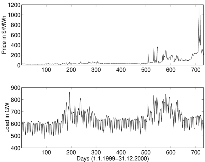
Figure 1: California Power Exchange daily average market clearing prices (top panel) and California power market daily system-wide load (bottom panel) since January 1st, 1999 until December 31st, 2000. The annual and weekly seasonalities are clearly visible.

The seasonality can be easily observed in the frequency domain by plotting a sample analogue of the spectral density, i.e. the periodogram

$$I_{n}(\omega_{k})=\frac{1}{n}\left|\sum_{t=1}^{n}x_{t}\exp\{-2\pi i(t-1)\omega_{k}\}\right|^{2},$$ (1)

where $\{x_{1},...,x_{n}\}$ is the vector of observations, $\omega_{k}=k/n$, $k=1,...,[n/2]$ and $[x]$ denotes the largest integer less then or equal to $x$. In the top panel of Fig. 2 we plotted the periodogram for the system-wide load. It shows well-defined peaks at frequencies corresponding to cycles with period 7 and 365 days. The smaller peaks close to $\omega_{k}=0.3$ and 0.4 indicate periods of 3.5 and 2.33 days, respectively. Both peaks are the so called harmonics (multiples of the 7-day period frequency) and indicate that the data exhibits a 7-day period but is not sinusoidal. The weekly period was also observed in lagged autocorrelation plots [14].

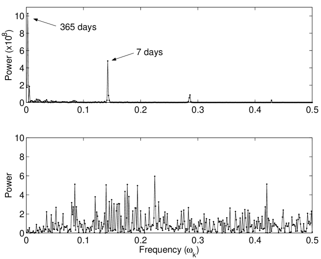
Figure 2: Periodogram of the California power market daily system-wide load since January 1st, 1999 until December 31st, 2000 (top panel). The annual and weekly frequencies are clearly visible. Periodogram of the load returns after removal of the weekly and annual cycles (bottom panel). No dominating frequency can be observed.

To remove the weekly cycle we used the moving average technique [5]. For the vector of daily loads $\{x_{1},...,x_{731}\}$ the trend was first estimated by applying a moving average filter specially chosen to eliminate the weekly component and to dampen the noise:

$$\hat{m}_{t}=\frac{1}{7}({x_{t-3}+...+x_{t+3}}),$$ (2)

where $t=4,...,728$. Next, we estimated the seasonal component. For each $k=1,...,7$, the average $w_{k}$ of the deviations $\{(x_{k+7j}-\hat{m}_{k+7j}),4\leq k+7j\leq 728\}$ was computed. Since these average deviations do not necessarily sum to zero, we estimated the seasonal component $s_{k}$ as

$$\hat{s}_{k}=w_{k}-\frac{1}{7}\sum_{i=1}^{7}w_{i},$$ (3)

where $k=1,...,7$ and $\hat{s}_{k}=\hat{s}_{k-7}$ for $k>7$. The deseasonalized (with respect to the 7-day cycle) data was then defined as

$$d_{t}=x_{t}-\hat{s}_{t}\quad\mbox{for $t=1,...,731$}.$$ (4)

Finally we removed the trend from the deseasonalized data $\{d_{t}\}$ by taking logarithmic returns $r_{t}=\log(d_{t+1}/d_{t})$, $t=1,...,730$.

After removing the weekly seasonality we were left with the annual cycle. Unfortunately, because of the short length of the time series (only two years), the method applied to the 7-day cycle could not be used to remove the annual seasonality. To overcome this we applied a new method which consists of the following [15]:

(i)

calculate a 25-day rolling volatility [8] for the whole vector $\{r_{1},...,r_{730}\}$;

(ii)

calculate the average volatility for one year, i.e. in our case

$$v_{t}=\frac{v_{t}^{1999}+v_{t}^{2000}}{2};$$ (5)

(iii)

smooth the volatility by taking a 25-day moving average of $v_{t}$;

(iv)

finally, rescale the returns by dividing them by the smoothed annual volatility.

The obtained time series (see the top panel of Fig. 3) showed no apparent trend and seasonality (see the bottom panel of Fig. 2). Therefore we treated it as a realization of a stationary process. Moreover, the dependence structure exhibited only short-range correlations. Both, the autocorrelation function (ACF) and the partial autocorrelation function (PACF) rapidly tend to zero (see the bottom panels of Fig. 3), which suggests that the deseasonalized load returns can be modeled by an ARMA-type process.

3 Modeling with ARMA processes

The mean-corrected (i.e. after removing the sample mean=0.0010658) deseasonalized load returns were modeled by ARMA (Autoregressive Moving Average) processes

$$X_{t}-\phi_{1}X_{t-1}-...-\phi_{p}X_{t-p}=Z_{t}+\theta_{1}Z_{t-1}+...+\theta_{q}Z_{t-q},\quad t=1,...,n,$$ (6)

where $(p,q)$ denote the order of the model and $\{Z_{t}\}$ is a sequence of independent, identically distributed variables with mean 0 and variance $\sigma^{2}$ (denoted by $\mbox{iid}(0,\sigma^{2})$ in the text).

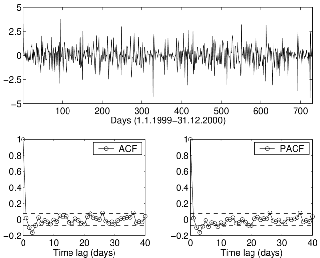
Figure 3: Load returns after removal of the weekly and annual cycles (top panel). The ACF (bottom left panel) and PACF (bottom right panel) for the mean-corrected deseasonalized load returns. Dashed lines represent the bounds $\pm 1.96/\sqrt{730}$, i.e. the 95% confidence intervals of Gaussian white noise.

The maximum likelihood estimators $\hat{\phi}=(\hat{\phi_{1}},...,\hat{\phi_{p}})$, $\hat{\theta}=(\hat{\theta_{1}},...,\hat{\theta_{q}})$ and $\hat{\sigma}^{2}$ of the parameters $\phi=(\phi_{1},...,\phi_{p})$, $\theta=(\theta_{1},...,\theta_{q})$ and $\sigma^{2}$, respectively, were obtained after a preliminary estimation via the Hannan-Rissanen method [5] using all 730 deseasonalized returns. The parameter estimates and the model size ($p$, $q$) were selected to be those that minimize the bias-corrected version of the Akaike criterion, i.e. the AICC statistics

$$\mbox{AICC}=-2\ln L+\frac{2(p+q+1)n}{n-p-q-2},$$ (7)

where $L$ denotes the maximum likelihood function and $n=730$.

The optimization procedure led us to the following ARMA(1,6) model (with $\theta_{4}=\theta_{5}=0$)

$$X_{t} = 0.332776X_{t-1}+$$ (8)

$$+Z_{t}-0.383245Z_{t-1}-0.12908Z_{t-2}-0.149307Z_{t-3}-0.0531862Z_{t-6},$$

where $t=1,...,730$ and $\{Z_{t}\}\sim$ iid$(0,0.838716)$. The value of the AICC criterion obtained for this model was AICC=1956.294.

In order to check the goodness of fit of the model to the set of data we compared the observed values with the corresponding predicted values obtained from the fitted model. If the fitted model was appropriate, then the residuals

$$\hat{W}_{t}=\frac{X_{t}-\hat{X}_{t}(\hat{\phi},\hat{\theta})}{\sqrt{\varsigma_{t-1}(\hat{\phi},\hat{\theta})}},\quad t=1,...,730,$$ (9)

where $\hat{X}_{t}(\hat{\phi},\hat{\theta})$ denotes the predicted value of $X_{t}$ based on $X_{1},...,X_{t-1}$ and $\varsigma_{t-1}=E(X_{t}-\hat{X}_{t})^{2}/\sigma^{2}$, should behave in a manner that is consistent with the model. In our case this means that the properties of the residuals should reflect those of an iid noise sequence with mean 0 and variance $\sigma^{2}$.

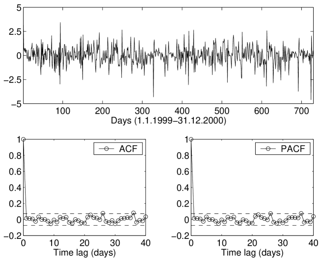
Figure 4: The residuals obtained from the ARMA(1,6) model (top panel). The ACF (bottom left panel) and the PACF (bottom right panel) of the residuals. Dashed lines represent the bounds $\pm 1.96/\sqrt{730}$.

The residuals obtained from the ARMA(1,6) model fitted to the mean-corrected deseasonalized load returns are displayed in the top panel of Fig. 4. The graph gives no indication of a nonzero mean or nonconstant variance. The sample ACF and PACF of the residuals fall between the bounds $\pm 1.96/\sqrt{730}$ indicating that there is no correlation in the series, see the bottom panels of Fig. 4. Recall that for large sample size $n$ the sample autocorrelations of an iid sequence with finite variance are approximately iid with distribution $N(0,1/n)$. Therefore there is no reason to reject the fitted model on the basis of the autocorrelation or partial autocorrelation function. However, we should not rely only on simple visual inspection techniques. For our results to be more statistically sound we performed several standard tests for randomness. The results of the portmanteau, turning point, difference-sign and rank tests are presented in Table 1. Short descriptions of all applied tests can be found in the Appendix.

Table 1: Test statistics and p-values for the residuals.

Test	Test statistics value	p-value
Portmanteau	15.03	(0.7747)
Turning point	464	(0.0609)
Difference-sign	361	(0.6536)
Rank	131090	(0.5529)

As we can see from Table 1, if we carry out the tests at commonly used 5% level, the tests do not detect any deviation from the iid behavior. Thus there is not sufficient evidence to reject the iid hypothesis. Moreover, the order $p=0$ of the minimum AICC autoregressive model for the residuals also suggests the compatibility of the residuals with white noise, see the Appendix. Therefore we may conclude that the ARMA(1,6) model (defined by eq. (8)) fits the mean-corrected deseasonalized load returns very well.

4 Distribution of the residuals

In the previous Section we showed that the residuals are a realization of an iid(0,$\sigma^{2}$) sequence. But what precisely is their distribution? The answer to this question is important, because if the noise distribution is known then stronger conclusions can be drawn when a model is fitted to the data. There are simple visual inspection techniques that enable us to check whether it is reasonable to assume that observations from an iid sequence are also Gaussian. The most widely used is the so-called normal probability plot, see Fig. 5. If the residuals were Gaussian then they would form a straight line. Obviously they are not Gaussian – the deviation from the line is apparent. This deviation suggests that the residuals have heavier tails.

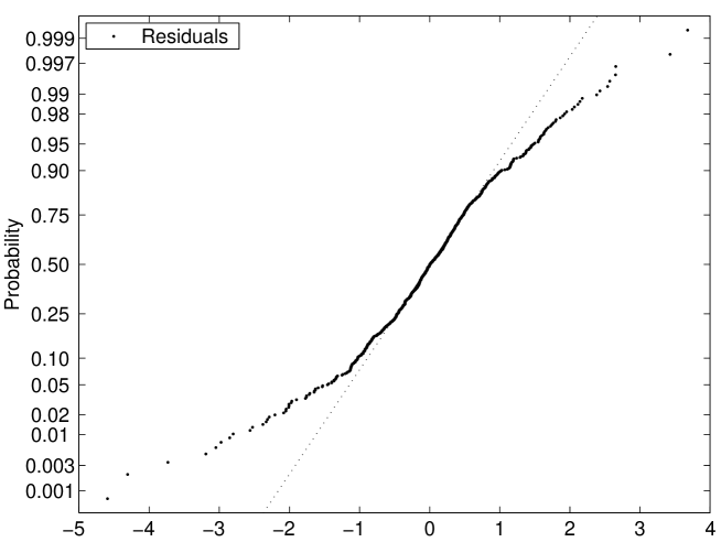
Figure 5: The normal probability plot of the residuals obtained from the ARMA(1,6) model. If the residuals were Gaussian then they would form a straight line.

However, we have to bear in mind that in order to comply with the ARMA model assumptions the distribution of the residuals must have a finite second moment. In the class of heavy-tailed laws with finite variance the hyperbolic distribution seems to be a natural candidate.

The hyperbolic law was introduced by Barndorff-Nielsen [1] for modeling the grain size distribution of windblown sand. It was also found to provide an excellent fit to the distributions of daily returns of stocks from a number of leading German enterprises [6, 10]. The name of the distribution is derived from the fact that its log-density forms a hyperbola. Recall that the log-density of the normal distribution is a parabola. Hence the hyperbolic distribution provides the possibility of modeling heavy tails.

The hyperbolic distribution is defined as a normal variance-mean mixture where the mixing distribution is the Inverse Gaussian law. More precisely, a random variable has the hyperbolic distribution if its density is of the form

$$f(x;\alpha,\beta,\delta,\mu)=\frac{\sqrt{\alpha^{2}-\beta^{2}}}{2\alpha\delta K_{1}(\delta\sqrt{\alpha^{2}-\beta^{2}})}\exp\left\{-\alpha\sqrt{\delta^{2}+(x-\mu)^{2}}+\beta(x-\mu)\right\},$$ (10)

where the normalizing constant $\mbox{K}_{1}(t)=\frac{1}{2}\int_{0}^{\infty}\exp\{-\frac{1}{2}t(x+\frac{1}{x})\}dx$, $t>0$, is the modified Bessel function with index 1, the scale parameter $\delta>0$, the location parameter $\mu\in R$ and $0\leq|\beta|<\alpha$. The latter two parameters – $\alpha$ and $\beta$ – determine the shape, with $\alpha$ being responsible for the steepness and $\beta$ for the skewness.

Given a sample of independent observations all four parameters can be estimated by the maximum likelihood method. In our studies we used the ’hyp’ program [3] to obtain the following estimates

$$\hat{\alpha}=1.671304,\qquad\hat{\beta}=-0.098790,\qquad\hat{\delta}=0.298285,\qquad\hat{\mu}=0.076975.$$

The empirical probability density function (PDF) – to be more precise: a kernel estimator of the density – together with the estimated hyperbolic PDF are presented in Fig. 6. We can clearly see that, on the semi-logarithmic scale, the tails of the residuals’ density form straight lines, which justifies our choice of the theoretical distribution. The adjusted Kolmogorov statistics $K=\sqrt{n}\sup_{x}|F(x)-F_{n}(x)|$, where $F(x)$ is the theoretical and $F_{n}(x)$ is the empirical cummulative distribution function, returns the value $K=1.5652$. This indicates that there is not sufficient evidence to reject the hypothesis of the hyberbolic distribution of the residuals at the 1% level. For comparison we fitted a Gaussian law to the residuals as well. In this case the adjusted Kolmogorov statistics returned $K=1.8019$ causing us to reject the Gaussian hypothesis of the residuals at the same level.

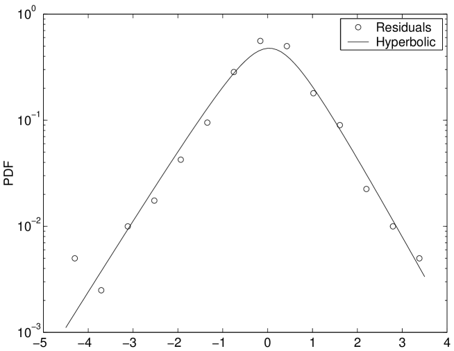
Figure 6: The empirical probability density function (a kernel estimator of the density) and the approximating hyperbolic PDF on the semi-logarithmic scale.

5 Conclusions

Due to limited monitoring in a power distribution system its loads usually are not known in advance and can only be forecasted based on the available information. In this paper we showed that it is possible to model deseasonalized loads via ARMA processes with heavy-tailed hyperbolic noise. This method could be used to forecast loads in a power market. Its effectiveness, however, still has to be tested and will be the subject of our further research.

Appendix: Tests for randomness

The portmanteau test.

Instead of checking to see if each sample autocorrelation $\hat{\rho}(j)$ falls inside the bounds $\pm 1.96/\sqrt{n}$, where $n$ is the sample size, it is possible to consider a single statistic introduced by Ljung and Box [11] $Q=n(n+2)\sum_{j=1}^{h}\hat{\rho}^{2}(j)/(n-j)$, whose distribution can be approximated by the $\chi^{2}$ distribution with $h$ degrees of freedom. A large value of $Q$ suggests that the sample autocorrelations of the observations are too large for the data to be a sample from an iid sequence. Therefore we reject the iid hypothesis at level $\alpha$ if $Q>\chi^{2}_{1-\alpha}(h)$, where $\chi^{2}_{1-\alpha}$ is the $(1-\alpha)$ quantile of the $\chi^{2}$ distribution with $h$ degrees of freedom.

The turning point test.

If $y_{1},...,y_{n}$ is a sequence of observations, we say that there is a turning point at time $i$ ($1<i<n$) if $y_{i-1}<y_{i}$ and $y_{i}>y_{i+1}$ or if $y_{i-1}>y_{i}$ and $y_{i}<y_{i+1}$. In order to carry out a test of the iid hypothesis (for large $n$) we denote the number of turning points by $T$ ($T$ is approximately $N(\mu_{T},\sigma^{2}_{T})$, where $\mu_{T}=2(n-2)/3$ and $\sigma^{2}_{T}=(16n-29)/90$) and we reject this hypothesis at level $\alpha$ if $|T-\mu_{T}|/\sigma_{T}>\Phi_{1-\alpha/2}$, where $\Phi_{1-\alpha/2}$ is the $(1-\alpha/2)$ quantile of the standard normal distribution. The large value of $T-\mu_{T}$ indicates that the series is fluctuating more rapidly than expected for an iid sequence; a value of $T-\mu_{T}$ much smaller than zero indicates a positive correlation between neighboring observations.

The difference-sign test.

For this test we count the number $S$ of values $i$ such that $y_{i}>y_{i-1}$, $i=2,...,n$. For an iid sequence and for large $n$, $S$ is approximately $N(\mu_{S},\sigma^{2}_{S})$, where $\mu_{S}=(n-1)/2$ and $\sigma^{2}_{S}=(n+1)/12$. A large positive (or negative) value of $S-\mu_{S}$ indicates the presence of an increasing (or decreasing) trend in the data. We therefore reject the assumption of no trend in the data if $|S-\mu_{S}|/\sigma_{S}>\Phi_{1-\alpha/2}$.

The rank test.

The rank test is particularly useful for detecting a linear trend in the data. We define $P$ as the number of pairs $(i,j)$ such that $y_{j}>y_{i}$ and $j>i$, $i=1,...,n-1$. For an iid sequence and for large $n$, $P$ is approximately $N(\mu_{P},\sigma^{2}_{P})$, where $\mu_{P}=n(n-1)/4$ and $\sigma^{2}_{P}=n(n-1)(2n+5)/72$. A large positive (negative) value of $P-\mu_{P}$ indicates the presence of an increasing (decreasing) trend in data. The iid hypothesis is therefore rejected at level $\alpha$ if $|P-\mu_{P}|/\sigma_{P}>\Phi_{1-\alpha/2}$.

The minimum AICC AR model test.

A simple test for whiteness of a time series is to fit autoregressive models of orders $p=0,1,...,p_{max}$, for some large $p_{max}$, and to record the value of $p$ for which the AICC value attains the minimum. Compatibility of these observations with white noise is indicated by selection of the value $p=0$.

References

- [1] O.E. Barndorff-Nielsen, Exponentially decreasing distributions for the logarithm of particle size, Proc. Royal Soc. London A 353 (1977) 401-419.
- [2] R. Bjorgan, C.-C. Liu, J. Lawarree, Financial Risk Management in a Competitive Electricity Market, IEEE Trans. Power Systems 14 (1999) 1285-1291.
- [3] P. Blaesild, M. Sørensen, ’Hyp’ – a computer program for analyzing data by means of the hyperbolic distribution, Research Report no. 248, Univ. Aarhus, Dept. Theor. Statist. (1992).
- [4] S. Borenstein, The Trouble With Electricity Markets (and some solutions), POWER Working Paper PWP-081, UCEI (2001).
- [5] P.J. Brockwell, R.A. Davis, Introduction to Time Series and Forecasting, Springer-Verlag, New York, 1996.
- [6] E. Eberlein, U. Keller, Hyperbolic distributions in finance, Bernoulli 1 (1995) 281-299.
- [7] International Chamber of Commerce, Liberalization and privatization of the Energy Sector, Paris, July 1998.
- [8] V. Kaminski, The Challenge of Pricing and Risk Managing Electricity Derivatives, in ”The US Power Market”, Risk Books, London, 1997.
- [9] V. Kaminski, ed., Managing Energy Price Risk, 2nd. ed., Risk Books, London, 1999.
- [10] U. Küchler, K. Neumann, M. Sørensen, A. Streller, Stock returns and hyperbolic distributions, Discussion Paper no. 23, Humbolt University, Berlin (1994).
- [11] G.M. Ljung, G.E.P. Box, On a measure of lack of fit in time series models, Biometrica 65 (1978) 297-303.
- [12] G.S. Masson, Competitive Electricity Markets Around the World: Approaches to Price Risk Management, in [9], 1999.
- [13] S. Stoft, The market flaw California overlooked, New York Times, Jan. 2, 2001.
- [14] R. Weron, Energy price risk management, Physica A 285 (2000) 127-134.
- [15] R. Weron, B. Kozłowska, J. Nowicka-Zagrajek, Modeling electricity loads in California: a continuous-time approach, arXiv: cond-mat/0103257, to appear in Physica A (2001) Proceedings of the NATO ARW on Application of Physics in Economic Modelling.
- [16] C.D. Wolfram, Electricity Markets: Should the Rest of the World Adopt the UK Reforms?, POWER Working Paper PWP-069, UCEI (1999).