Statistical mechanics of secondary structures formed by random RNA sequences

Abstract

The formation of secondary structures by a random RNA sequence is studied as a model system for the sequence-structure problem omnipresent in biopolymers. Several toy energy models are introduced to allow detailed analytical and numerical studies. First, a two-replica calculation is performed. By mapping the two-replica problem to the denaturation of a single homogeneous RNA in $6$-dimensional embedding space, we show that sequence disorder is perturbatively irrelevant, i.e., an RNA molecule with weak sequence disorder is in a molten phase where many secondary structures with comparable total energy coexist. A numerical study of various models at high temperature reproduces behaviors characteristic of the molten phase. On the other hand, a scaling argument based on the extremal statistics of rare regions can be constructed to show that the low temperature phase is unstable to sequence disorder. We performed a detailed numerical study of the low temperature phase using the droplet theory as a guide, and characterized the statistics of large-scale, low-energy excitations of the secondary structures from the ground state structure. We find the excitation energy to grow very slowly (i.e., logarithmically) with the length scale of the excitation, suggesting the existence of a marginal glass phase. The transition between the low temperature glass phase and the high temperature molten phase is also characterized numerically. It is revealed by a change in the coefficient of the logarithmic excitation energy, from being disorder dominated to entropy dominated.

I Introduction

RNA is an important biopolymer critical to all living systems rnagen and may be the crucial entity in prebiotic evolution rna . Like for DNA, there are four types of nucleotides (or bases) A, C, G, and U which, when polymerized can form double helical structures consisting of stacks of stable Watson-Crick pairs (A with U or G with C). However unlike a long polymer of DNA, which is often accompanied by a complementary strand and forms otherwise featureless double helical structures, a polymer of RNA usually “operates” in the single-strand mode. It bends onto itself and forms elaborate spatial structures in order for bases located on different parts of the backbone to pair with each other, similar conceptually to how the sequence of an amino acid encodes the structure of a protein.

Understanding the encoding of structure from the primary sequence has been an outstanding problem of theoretical biophysics. Most theoretical work in the past decade have been focused on the problem of protein folding, which is very difficult analytically and numerically dill95 ; woly97 ; gare97 ; shak97 . Here, we study the problem of RNA folding, specifically the formation of RNA secondary structures. For RNA, the restriction to secondary structures is meaningful due to a separation of energy scales. It is this restriction that makes the RNA folding problem amenable to detailed analytical and numerical studies higg00 . There exist efficient algorithms to compute the exact partition function of RNA secondary structures zuke81 ; mcca90 ; hofa94 . Together with the availability of carefully measured free energy parameters frei86 describing the formation of various microscopic structures (e.g., stacks, loops, hairpins, etc.), the probable secondary structures formed by any given RNA molecule of up to a few thousand bases can be obtained readily. On the experimental side, RNA molecules of $10^{2}$ – $10^{5}$ bases in length are available. Furthermore, the restriction to secondary structures can be physically enforced in a salt solution with monovalent ions, e.g., ${\rm Na}^{+}$, so that controlled experiments are in principle possible tino99 .

In this work, we are not concerned with the structure formed by a specific sequence. Instead, we will study the statistics of secondary structures formed by the ensemble of long random RNA sequences (of at least a few thousand bases in length in practice). Such knowledge may be of value in detecting important structural components in messenger RNAs which may otherwise be regarded as random from the structural perspective, in understanding how functional RNAs arise from random RNA sequences rna , or in characterizing the response of a long single-stranded DNA molecule to external pulling forces maie00 . More significantly from the theoretical point of view, the RNA secondary structure problem presents a rare tractable model of a random heteropolymer where concrete progress can be made regarding the thermodynamic properties higg00 ; dege68 ; higg96 ; bund99 ; pagn00 ; hart01 ; pagn01 . Nevertheless, there are many gaps in our understanding. This paper is a detailed report of our on-going effort in this regard. It provides a self-contained introduction of the random RNA problem to statistical physicists as a novel problem of disordered systems, and depicts several approaches we have tried to characterize this system.

The manuscript is organized as follows: In Sec. II, we provide a detailed introduction to the phenomenology of RNA secondary structure formation. We review the key simplifications which form the basis of efficient computing as well as exact solutions in some cases. We also review the properties of the “molten phase”, which is the simplest possible phase of the system assuming sequence disorder is not relevant. In Sec. III, we consider the effect of sequence disorder at high temperatures. We show numerical evidence that the random RNA sequence is in the molten phase at sufficiently high temperatures, and support this conclusion by solving the two-replica system which can be regarded as a perturbative study on the stability of the molten phase. In Sec. IV, we provide a scaling argument, and show why the molten phase should break down at low enough temperatures. This is followed by a detailed numerical study of the low temperature regime. We apply the droplet picture and characterize the statistics of large-scale, low-energy excitations of the secondary structures from the ground state structure. Our results support the existence of a very weak (i.e., marginal) glass phase characterized by logarithmic excitation energies. Finally, we describe the intermediate temperature regime where the system makes the transition from the glass phase to the molten phase. The solution of the two-replica problem is relegated to the appendices. We present two approaches: In Appendix A, we provide a mapping of the two-replica problem to the denaturation of an effective single RNA in $6$-dimensional embedding space; this approach highlights the connection of the RNA problem to the self-consistent Hartree theory and should be most natural to field theorists. In Appendices B and C, we present the exact solution. It is hoped that the two-replica solution may be helpful in providing the intuition needed to tackle the full $n$-replica problem.

II Review of RNA secondary structure

II.1 Model and definitions

II.1.1 Secondary structures

The secondary structure of an RNA describes the configuration of base pairings formed by the polymer. If the pairing of the $i^{\rm th}$ and $j^{\rm th}$ bases in a polymer of $N$ total bases is denoted by $(i,j)$ with $1\leq i<j\leq N$, then each secondary structure $S$ is defined by a list of such pairings, with each position appearing at most once in the list, and with the pairs subject to a certain restriction to be described shortly below. Each such structure can be represented by a diagram as shown in Fig. 1, where the solid line symbolizes the backbone of the molecule and the dashed lines stand for base pairings. The structure shown can be divided into stems of consecutive base pairs and loops which connect or terminate these stems. In naturally occurring RNA molecules, the stems typically comprise on the order of five base pairs. They locally form the same double helical structure as DNA molecules. However, while the latter typically occur in complementary pairs and bind to each other, RNA molecules are mostly single-stranded and hence must fold back onto themselves in order to gain some base pairings.

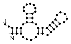
Figure 1: Diagramatic representation of an RNA secondary structure: The solid line symbolizes the backbone of the molecule while the dashed lines stand for the hydrogen-bonded base pairs formed. The backbone is shaped such that stems of subsequent base pairs and the loops connecting or terminating them can be clearly seen. These stems form double helical structures similar to that of DNA.

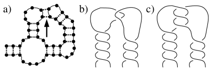
Figure 2: Pseudo-knots in RNA structures: The base pairings indicated by the arrow in (a) create a pseudo-knot. We exclude such configurations in our definition of secondary structures: The short pseudo-knots (called “kissing hairpins”) as shown in (b) do not contribute much to the total binding energy, and the long ones shown in (c) are kinetically forbidden since the double helical structure would require threading one end of the molecule through its loops many times.

By a secondary structure, one often considers only the restricted set of base pairings where any two base pairs $(i,j)$ and $(k,l)$ in a given secondary structure are either independent, i.e., $i<j<k<l$, or nested, i.e., $i<k<l<j$. This excludes the so-called pseudo-knots (as exemplified by Fig. 2) and makes analytical and numerical studies much more tractable. For an RNA molecule, the exclusion of pseudo-knots is a reasonable approximation because the long pseudo-knots are kinetically difficult to form, and even the short ones occur infrequently in natural RNA structures tino99 . The latter is due to their relatively low binding energies for short sequences and the strong electrostatic repulsion of the backbone — because the polymer backbone is highly charged and pseudo-knotted configurations increase the density of the molecule, their formation can be relatively disfavored in low salt solution. Similarly, the tertiary structures which involve additional interactions of paired bases are strongly dependent on electrostatic screening and can be “turned off” experimentally by using monovalent salt solution tino99 . Indeed, the pseudo-knots are often deemed part of the tertiary structure of an RNA molecule. Throughout this study, we will exclude pseudo-knots in our definition of secondary structures. Without the pseudo-knots, a secondary structure can alternatively be represented by a diagram of non-crossing arches or by a “mountain” diagram as shown in Fig. 3.

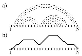
Figure 3: Abstract representations of the RNA secondary structure shown in Fig. 1: In (a) the solid line symbolizes the stretched out backbone of the molecule while the dashed arches stand for the base pairs formed. Due to the no pseudo-knot constraint two arches never cross. (b) shows an equivalent representation as a “mountain diagram”. It is a line derived from the arch diagram by going along the backbone from left to right and going one step up for every beginning arch, horizontally for each unbound base, and one step down for each ending arch. Such a mountain always stays above the baseline and comes back to the baseline at base $N$.

II.1.2 Interaction energies

In order to calculate Boltzmann factors within an ensemble of secondary structures, we need to assign an energy $E[S]$ to each structure $S$. Each secondary structure can be decomposed into elementary pieces such as the stems of base pairs and the connecting loop regions as shown in Fig. 1. A common approach is to assume that the contributions from these structural elements to the total energy are independent of each other and additive.

Within a stem of base pairs, the largest energy contribution is the stacking energy between two adjacent base pairs (G-C, A-U, or G-U), and the total energy of the stem is the sum of stacking energies over all adjacent base pairs. Since each secondary structure is defined as a single state in our ensemble, it is necessary to integrate out all other microscopic degrees of freedom of the bases within a given secondary structure and use an effective energy parameter for each base stacking. The most convenient one to use is the Gibbs free energy of stacking frei86 , which contains an enthalpic term due to base stacking, and an entropic term due to the loss of single-stranded degrees of freedom (as well as the additional conformational change of the backbone and even the surrounding water molecules) due to base pairing. The magnitudes of these stacking free energies actually depend on the identity of all four bases forming the two base pairs bracketing the stack and are dependent on temperature themselves. While their typical values are on the order of $k_{\mathrm{B}}T$ at room temperature, the enthalpic and entropic contributions are each on the order of $10k_{\mathrm{B}}T$. Thus, upon moderately increasing the temperature from room temperature to about $80^{\circ}C$, the stacking free energies become repulsive and the RNA molecule denatures.

The stacking free energies account for most but not all of the entropic terms for a given secondary structure. There is an additional (logarithmic) “loop energy” term associated with the entropy loss of each closed loop of single-stranded RNA formed by the secondary structure, as well as the energy necessary to bend the single strand. All of these energy parameters have been measured in great detail frei86 . When incorporated into an efficient dynamic programming algorithm (to be described below), they can rather successfully predict the secondary structures of many RNA molecules of up to several hundred bases in length zuke81 ; mcca90 ; hofa94 .

In this paper, we investigate the statistical properties of long, random RNA sequences far below the denaturation temperature. We are interested in generic issues such as the existence of a glass phase and various scaling properties. Guided by experiences with other disordered systems youn98 , we believe these generic properties of the system should not depend on the specific choice of the model details. Since the full model used in Refs zuke81 ; mcca90 ; hofa94 makes analytical and numerical studies unnecessarily clumsy, we will examine a number of simplified models, while preserving the most essential feature of the system, namely, the pattern of matches and mismatches between different positions of the sequence.

As in the realistic model described above, we choose our reference energy to be the unbound state, so that each unbound base in a secondary structure is assigned the energy $0$. We will neglect the logarithmic loop energy, which is important very close to the denaturation transition moro01 where the average binding energy is close to zero, but not far below the denaturation temperature where most bases are paired. Moreover, we will radically simplify the energy rules for base pairing: We neglect the stacking energies and instead associate an interaction energy $\varepsilon_{i,j}$ with every pairing $(i,j)$. Thus,

$$E[S]=\sum_{(i,j)\in S}\varepsilon_{i,j}$$ (1)

is the total energy of the structure $S$.

Within this model, it remains to be decided how to choose the energy parameters $\varepsilon_{i,j}$’s. One possibility is to choose each of the bases $b_{1}\ldots b_{N}$ randomly from the ‘alphabet’ set $\{A,C,G,U\}$ and then assign

$$\varepsilon_{i,j}=\left\{\begin{array}[]{rl}-u_{\mathrm{m}}&\mbox{$b_{i}$--$b_{j}$ is a Watson-Crick base pair}\\ u_{\mathrm{mm}}&\mbox{otherwise}\end{array}\right.$$ (2)

with $u_{\mathrm{m}},u_{\mathrm{mm}}>0$ being the match or mismatch energy respectively. Here, the value of $u_{\mathrm{mm}}$ is actually not essential as long as it is repulsive, since the two bases always have the energetically preferred option to not bind at all. Thus the energetics of the system is set by $u_{\mathrm{m}}$. In our numerical study to be reported in Secs. III and IV, we will primarily use this model with $u_{\mathrm{m}}=u_{\mathrm{mm}}=1$. We will refer to this as the “sequence disorder” model.

For analytical calculations, it is preferable to treat all the $\varepsilon_{i,j}$’s as independent identically distributed random variables, i.e., to assume

$$\rho[\{\varepsilon_{i,j}\}]=\prod_{1\leq i<j\leq N}\rho(\varepsilon_{i,j})$$ (3)

for the joint distribution function $\rho[\{\varepsilon_{i,j}\}]$ of all the $\varepsilon_{i,j}$’s. This choice neglects the correlations between $\varepsilon_{i,j}$ and $\varepsilon_{i,k}$ which are generated through the shared base $b_{i}$; it is an additional approximation on the model (2). However, we do not anticipate universal quantities to depend on such subtle correlation of the $\varepsilon_{i,j}$’s. This will be tested numerically by comparing the behavior of the model (2) with that of the model defined by Eq. (3) together with

$$\rho(\varepsilon)=\frac{1}{4}\delta(\varepsilon+u_{\mathrm{m}})+\frac{3}{4}\delta(\varepsilon-u_{\mathrm{mm}}).$$ (4)

This distribution is chosen to mimic the random sequence model (2) with a 4-letter alphabet, but it does not contain any correlation between the different $\varepsilon_{i,j}$’s. We will refer to this model as defined by Eqs. (3) and (4) as the “energy disorder” model.

In the actual analytical calculations, we will go even one step further and take the $\varepsilon_{i,j}$ to be Gaussian random variables specified by

$$\rho(\varepsilon)=\frac{1}{\sqrt{2\pi D}}\,e^{-(\varepsilon-\overline{\varepsilon})^{2}/2D}$$ (5)

where $\overline{\varepsilon}$ is the average binding energy and $D$ is the variance. In this model (referred to below as “Gaussian disorder” model,) the parameter $D$ provides us with a convenient measure of the disorder strength. Again, universal quantities should not depend on the choice of the distribution functions. We will test this directly by performing numerical studies for these Gaussian random energies, with

$$\overline{\varepsilon}=-\frac{1}{4}u_{\mathrm{m}}+\frac{3}{4}u_{\mathrm{mm}}\quad\mbox{and}\quad D=\frac{3}{16}(u_{\mathrm{m}}+u_{\mathrm{mm}})^{2}$$ (6)

chosen to match the first two moments of the distribution Eq. (4).

In contrast to prior numerical studies pagn00 , we do not exclude base pairing between neighboring bases $(i,i+1)$, i.e., we do not set a minimal allowed length for the hairpins. Setting a constraint on the minimal hairpin length would make the analytical study much more cumbersome. However, in the study by Pagnani et al. pagn00 , it has been argued that the system will not be frustrated (and hence will not form a glass) without this additional constraint. We believe this is an artifact of the 2-letter alphabet used by Pagnani et al. in order to generate the binding energy $\varepsilon_{i,j}$’s via a rule similar to Eq. (2): It is simple to see that for any 2-letter sequence in which the like letters repel and unlike letters attract, one can always find the minimal total binding energy by pairing up neighboring bases of opposite types and removing them from the sequence if no additional constraints such as the minimal hairpin length are enforced. As we will discuss in detail in Sec. IV.1 this is not a problem if the alphabet size is larger than 2. Thus, in our study, we use the sequence disorder model with a 4-letter alphabet, or the energy disorder model, without enforcing the minimal hairpin length constraint. While the minimal hairpin length (of 3 bases) is known for real RNA folding, it should not change the universal properties of long RNA sequences.

II.1.3 Partition function

Once the energy of each secondary structure is defined, we can study the partition function

$$Z(N)=\sum_{S\in{\bf S}(N)}e^{-\beta E[S]}$$ (7)

of the molecule where ${\bf S}(N)$ denotes the set of all allowed secondary structures of a polymer of $N$ bases, and $\beta=1/k_{B}T$. To calculate this partition function, it is useful to study the restricted partition function $Z_{i,j}$ of the substrand from position $i$ to position $j$ of the RNA molecule. Given the model (1), the restricted partition functions can be split up according to the possible pairings of position $j$. This leads to the recursive equation higg96 ; dege68 ; wate78

$$Z_{i,j}=Z_{i,j-1}+\sum_{k=i}^{j-1}Z_{i,k-1}\cdot e^{-\beta\varepsilon_{k,j}}\cdot Z_{k+1,j-1}$$ (8)

with $Z(N)=Z_{1,N}$ being the total partition function of the molecule. In terms of the arch diagrams introduced in Fig. 3(a) this can be represented as

(9)

where the wavy lines stand for the restricted partition functions. This is easily recognized as a Hartree equation. Since the restricted partition functions on the right hand side of this equation all correspond to shorter pieces of the RNA molecule than the left hand side, this equation allows one to calculate the exact partition function of an RNA molecule of length $N$ with arbitrary interactions $\varepsilon_{i,j}$ in $O(N^{3})$ time. This is accomplished by starting with the partition functions for single bases and recursively applying Eq. (8), and is known as a dynamic programming algorithm mcca90 ; wate78 . This algorithm allows one to compute numerically the partition function involving all secondary structures, for arbitrary RNA molecules of up to $N\approx 10,000$ bases. It also forms the basis of analytical approaches to the problem as we will see shortly.

II.1.4 Physical observables

Apart from the partition function itself, we will use additional observables in order to characterize the behavior of RNA secondary structures. One such quantity of interest is the binding probability $P_{i,j}$, i.e., the probability that positions $i$ and $j$ are paired given the $\varepsilon_{i,j}$’s,

$$P_{i,j}\equiv\frac{e^{-\beta\varepsilon_{i,j}}Z_{i+1,j-1}Z_{j+1,i-1}}{Z_{1,N}}$$ (10)

where $Z_{i+1,j-1}$ is given by the recursion equation (8) and $Z_{j+1,i-1}$ is the partition function of the sequence $b_{j+1}b_{j+2}\ldots b_{N}b_{1}\ldots b_{i-2}b_{i-1}$. The latter can be calculated as the quantity $Z_{j+1,N+i-1}$ when applying the recursion Eq. (8) to the duplicated sequence $b_{1}\ldots b_{N}b_{1}\ldots b_{N}$. Thus, all $N(N-1)/2$ such constraint partition functions can be calculated with the same recursion in $O(N^{3})$ time. The logarithms

$$\Delta F_{i,j}=-k_{\mathrm{B}}T\ln P_{i,j}$$ (11)

of these binding probabilities have a natural interpretation: they can be read as the “pinching free energies”, i.e., as the free energy cost of a pinch between positions $i$ and $j$ and the unperturbed state. We will make extensive use of this concept of pinched structures in our discussion of the low temperature behavior of RNA secondary structures in Sec. IV. In our numerical investigations, we will choose as a representative of all the pinching energies for different positions by

$$\Delta F(N)\equiv\Delta F_{1,N/2+1}$$ (12)

which is the free energy cost of the largest possible pinch that splits the molecule of length $N$ into two pieces of length $N/2-1$ each.

Another quantity which describes a secondary structures is its “size profile”. As an intrinsic measure of the size of a given secondary structure $S$, we use the “ladder distance” $h_{i}(S)$ between the base at position $1$ and the base at position $i$, which is the the number of pairings (or ladders) one has to cross to go from a pair involving base $1$ to the base $i$; see Fig. 4. It can be defined for each secondary structure $S$ as the total number of pairings $(k,k^{\prime})\in S$ that bracket $i$, i.e.,

$$h_{i}(S)\equiv|\{(k,k^{\prime})\in S|k<i\leq k^{\prime}\}|.$$ (13)

This quantity can be very easily visualized as the “height” at position $i$ of the mountain representation of the secondary structure $S$ as shown in Fig. 3(b). A quantity characterizing the full ensemble of secondary structures is the thermal average $\langle h_{i}\rangle$ of this size profile over all secondary structures with their respective Boltzmann factors; it can be straightforwardly calculated from the probabilities $P_{k,k^{\prime}}$ as

$$\langle h_{i}\rangle=\sum_{k=1}^{i-1}\sum_{k^{\prime}=i}^{N}P_{k,k^{\prime}}.$$ (14)

Since we expect all positions in the sequence to behave in a similar way, in our numerics we will summarize the properties of the size profile by the ladder distance from the first to the middle base, i.e., we will study

$$\langle h\rangle\equiv\langle h_{N/2+1}\rangle$$ (15)

as a quantity representing the overall “size” of an ensemble of secondary structures.

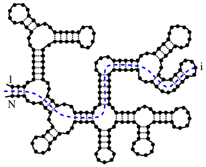
Figure 4: Definition of the “size profile” $h_{i}$ of a secondary RNA structure: The size profile measures the extension of the structure if drawn as a planar diagram. As an intrinsic definition of $h_{i}$ which captures this notion of the size of a secondary structure at position $i$, we use the “ladder distance” of base $i$ from the end of the molecule, i.e., the number of base pairs which have to be crossed when connecting position $i$ to position $1$ along the folded structure as indicated by the dashed line.

II.2 The molten phase

II.2.1 Definition of the molten phase

If sequence disorder does not play an important role, we may describe the RNA molecule by replacing all the binding energies $\varepsilon_{i,j}$ by some effective value $\varepsilon_{0}<0$. As we will see later, this will be an adequate description of our random RNA models at high enough temperatures (but before denaturation.) For the real RNAs, this provides a coarse grained description of repetitive, self-complementary sequences, e.g., CAGCAG…CAG, which are involved in a number of diseases mita97 . We will refer to RNA which is well described by this model without sequence disorder as being in the “molten” phase. It serves as a starting point for modeling non-specific self-binding of RNA molecules, and its properties will form the basis of our study of the random RNA at low temperatures.

II.2.2 Partition function

Since in the absence of sequence disorder, the energy of a structure $S$ depends only on the number of paired bases $|S|$ of this structure, we can write the partition function in the molten phase as

$$Z(N)=\sum_{S\in{\bf S}(N)}\exp\left[-\beta\varepsilon_{0}|S|\right]$$ (16)

The partition functions of the sub-strands $Z_{i,j}$ become translationally invariant and can be written as

$$Z_{i,j}=G(j-i+2)$$ (17)

where $G(N)$ is only a function of the length $N$. The recursion equation (8) then takes the form

$$G(N+1)=G(N)+q\sum_{k=1}^{N-1}G(k)\cdot G(N-k),$$ (18)

where

$$q\equiv e^{-\beta\varepsilon_{0}}.$$ (19)

Upon introducing the $z$-transform

$$\widehat{G}(z)=\sum_{N=1}^{\infty}G(N)z^{-N},$$ (20)

the convolution can be eliminated and the recursion equation turns into a quadratic equation

$$z\widehat{G}(z)-1=\widehat{G}(z)+q\widehat{G}^{2}(z)$$ (21)

with the solution

$$\widehat{G}(z)=\frac{z-1-\sqrt{(z-1)^{2}-4q}}{2q}.$$ (22)

Performing the inverse $z$-transformation in the saddle point approximation yields the expression dege68 ; bund99 ; wate78

$$G(N)\approx A_{0}(q)N^{-\theta_{0}}z_{0}^{N}(q)$$ (23)

in the limit of large $N$, with the exponent $\theta_{0}=3/2$ and the non-universal quantities $z_{0}(q)=1+2\sqrt{q}$ and $A_{0}(q)=[(1+2\sqrt{q})/4\pi q^{3/2}]^{1/2}$.

This result characterizes the state of the RNA where a large number of different secondary structures of equal energy coexist in the thermodynamic ensemble, and the partition function is completely dominated by the configurational entropy of these secondary structures. While the result is derived specifically for the special case $\varepsilon_{i,j}=\varepsilon_{0}$, we will argue below that it is applicable also to random $\varepsilon_{i,j}$’s at sufficiently high temperatures, in the sense that for long RNA molecules, the partition function is dominated by an exponentially large number of secondary structures all having comparable energies (within $O(k_{B}T)$) that are smoothly related to each other in configuration space. The latter is what we meant by the “molten phase”.

II.2.3 Scaling behavior

The exponent $\theta_{0}=3/2$ is an example of a scaling exponent characteristic of the molten phase. This and other exponents can be derived in a geometric way by the “mountain” representation of secondary structures as illustrated in Fig. 3(b). Each such mountain corresponds to exactly one secondary structure. In the molten phase, the weight of a secondary structure $S$ is simply given by $q^{|S|}$. This can be represented in the mountain picture by assigning a weight of $q^{1/2}$ to every upward and downward step and a weight of $1$ to every horizontal step. Since the only constraints on these mountains are (i) staying above the baseline, and (ii) returning to the baseline at the end, the partition function of an RNA of length $N$ is then simply that of a random walk of $N$ steps, constrained to start from and return to the origin, in the presence of a hard wall at the origin, with the above weights ($\sqrt{q}$ or $1$) assigned to each allowed step. This partition function is well-known to have the characteristic $N^{-3/2}$ behavior which we formally derived in the last section fell50 .

In this framework, it also becomes obvious why imposing a minimal hairpin length does not change the universal behavior of RNA at least in this molten phase: If the minimal allowed size of a hairpin is $s$, this enforces a potentially strong penalty for the formation of a hairpin, since with every hairpin $s$ bases are denied the possibility of gaining energy by base pairing. This tends to make branchings less favorable and thus leads to longer stems. However, this additional constraint translates in the mountain representation into the rule that an upwards step may not be followed by a downwards step within the next $s$ steps. This is clearly a local modification of the random walk. Thus, it does not change universal quantities although the above mentioned suppression of branchings will require much longer sequences in order to observe the asymptotic universal behavior. For real RNA parameters, the crossover length is very long due to this effect. For example, it is several hundred nucleotides for the CAG repeat, and even longer for some other repeats.

Another characteristic exponent describes the scaling of the ladder size $\langle h\rangle$ with the sequence length $N$. As already mentioned in its definition (15), $\langle h\rangle$ is equivalent to the average “height” of the mid-point of the sequence in the mountain picture. In the molten phase, the random walk analogy immediately yields the result

$$\langle h\rangle_{0}\sim N^{1/2},$$ (24)

where $\langle...\rangle_{0}$ denotes ensemble average in the molten phase.

As should be clear from the coarse-grained view depicted in Fig. 4, the ensemble of RNA secondary structures in the molten phase can be mapped directly to the ensemble of branched polymers. These branched polymers are rooted at the bases $i=1$ and $i=N$ of the RNA. In this context, $\theta_{0}=3/2$ is known as the configuration exponent of the rooted branched polymer lube81 . Additionally from the result (24), we see that the ladder length of the branched polymer scales as $N^{1/2}$. Because of the very visual analogy of the secondary structures to branched polymer, we refer to the configurational entropy of the secondary structures as the “branching entropy”.

Finally, the binding probabilities $P_{i,j}$ defined in Eq. (10) only depend on the distance $|i-j|$ in the molten phase, i.e., $P_{i,j}=p(|i-j|)$. The behavior of this function can be derived explicitly by inserting the result Eq. (23) for the partition function into Eq. (10). Alternatively, one just needs to recognize that $p(\ell)$ corresponds in the random walk analogy to the first-return probability of a random walk after $\ell$-steps. In either case, one finds the result

$$p(\ell)\sim\frac{\ell^{-\frac{3}{2}}(N-\ell)^{-\frac{3}{2}}}{N^{-\frac{3}{2}}},$$ (25)

i.e., the return probability decays with the separation $\ell$ of the two bases as a power law with the configuration exponent $\theta_{0}=3/2$. For the pinching free energy $\Delta F(N)$, we simply set $\ell=N/2$ and obtain

$$\Delta F_{0}=\frac{3}{2}k_{\mathrm{B}}T\ln N$$ (26)

for large $N$, i.e., it scales logarithmically in the molten phase. This logarithmic dependence merely reflects the loss in branching entropy due to the pinching constraint and is a manifestation of the configuration exponent $\theta_{0}=3/2$.

III Effect of Sequence Randomness: High Temperature Behavior

There are in principle three different scenaria for the behavior of long random RNA sequences. (i) Disorder is irrelevant at any finite temperature, so that the molten phase description presented in Sec. II.2 applies to long RNAs at all temperatures. (ii) Disorder is relevant at all temperatures, and the molten phase description would be completely inadequate. (iii) There is a finite temperature $T_{\mathrm{g}}$ above which the molten description of random RNA is correct, while below $T_{\mathrm{g}}$ a qualitatively different description is needed. In accordance with the statistical physics literature, we will refer to the non-molten phase as the glass phase, and $T_{\mathrm{g}}$ as the glass transition. The purpose of the study is to determine which of these three scenaria is actually realized, and to characterize the glass phase if either (ii) or (iii) is realized.

In this section, we study the high temperature behavior and demonstrate that the molten phase is stable with respect to weak sequence disorder. This ensures that the molten description of RNA given in Sec. II.2 is at least valid at high enough temperatures, thereby ruling out scenario (ii). We will address the question of whether there is a glass phase at low but finite temperatures in Sec. IV.

III.1 Numerics

Before we engage in detailed calculations, we want to convince ourselves with the help of some numerics that weak disorder does not destroy the molten phase. To this end, we study the observables introduced in Sec. II.1.4. We generate a large number of disorder configurations, i.e., interaction energies $\varepsilon_{i,j}$ using the 3 models introduced in Sec. II.1.2: sequence disorder, energy disorder, and Gaussian disorder as described by Eq. (2), Eqs. (3) and (4), and Eqs. (3) and (5) respectively, with $u_{\mathrm{m}}=u_{\mathrm{mm}}=1$. Then, we calculate the observables $\langle h\rangle$ and $\Delta F(N)$ for each disorder configuration at the relatively large temperature of $k_{B}T=2$ and average the obtained values over many disorder configurations. In order to keep the numerical effort manageable, we average over $10,000$ random sequences for $N\in\{10,20,40,80,160,320\}$, over $2,000$ sequences for $N=640$, and over $1,000$ sequences for $N=1,280$ and $N=2,560$.

Fig. 5 shows the results; disorder averaged quantities are denoted by an overline throughout the text. We see that the data for $\overline{\langle h\rangle}$ follows a power law with a fitted exponent $\overline{\langle h\rangle}\sim N^{0.54}$, with the exponent value decreasing for larger $N$’s. This result is consistent with the prediction Eq. (24) for the molten phase. Also, the pinching free energy follows the predicted logarithmic behavior Eq. (26) without any noticeable difference between the three choices of disorder. Taken together, these results indicate that the three models of disorder belong to the same universality class, i.e., the molten phase description of the uniformly attracting RNA, at high temperatures.

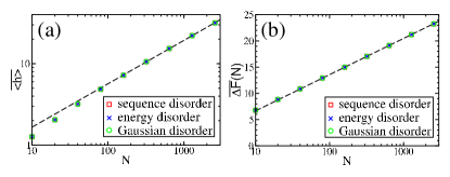
Figure 5: Scaling in the molten phase: These two plots show the dependence of several characteristic quantities of RNA secondary structures on the length $N$ of the sequence at $k_{B}T=2$. Each plot shows data for three different choices of disorder according to Eqs. (2), (4), and (5). (a) shows the scaling of the average size $\overline{\langle h\rangle}$ and the dashed line is the best fit $\overline{\langle h\rangle}\sim N^{0.54}$ to a power law. (b) shows the free energy of the largest pinch as defined in (12). The dashed line is up to an additive constant the logarithmic behavior $\frac{3}{2}\times 2\ln N$ predicted in Eq. (26). The statistical fluctuations are smaller than the size of the symbols in both plots. All plots suggest that the behavior of RNA secondary structures at high temperatures is well described by the molten phase picture and independent of the disorder.

III.2 The replica calculation

Now, we will establish the stability of the molten phase against weak disorder by an analytical argument. We will use Gaussian disorder characterized by Eqs. (3) and (5). As we have shown above, the different microscopic models of binding energies all yield the same scaling behaviors. With the uncorrelated Gaussian energies, it is possible to perform the ensemble average of the partition function $\overline{Z^{n}}$ of $n$ RNA molecules sharing the same disorder. The disorder-averaged free energy can then in principle be obtained via the “replica-trick” $\overline{\ln Z}=\lim_{n\to 0}(\overline{Z^{n}}-1)/n$, by solving the $n$-replica problem edwa75 .

The $n$-replica partition function can be written down formally as

$$\overline{Z^{n}} = \sum_{\{S_{1}\}}\ldots\sum_{\{S_{n}\}}\overline{\exp\left[-\sum_{k=1}^{n}\sum_{(i,j)\in S_{k}}\beta\varepsilon_{i,j}\right]}$$

$$= \sum_{\{S_{1}\}}\ldots\sum_{\{S_{n}\}}\prod_{k=1}^{n}\exp\left[-\beta\overline{\varepsilon}|S_{k}|\right]\exp\left[\frac{1}{2}\beta^{2}\sum_{k=1}^{n}\sum_{l=1}^{n}\sum_{(i,j)\in S_{k}}\sum_{(r,s)\in S_{l}}\overline{(\varepsilon_{i,j}-\overline{\varepsilon})(\varepsilon_{r,s}-\overline{\varepsilon})}\right]$$

$$= \sum_{\{S_{1}\}}\ldots\sum_{\{S_{n}\}}\prod_{k=1}^{n}\exp\left[-\beta\overline{\varepsilon}|S_{k}|\right]\exp\left[\frac{1}{2}\beta^{2}D\sum_{k=1}^{n}\sum_{l=1}^{n}|S_{k}\cap S_{l}|\right]$$

$$= \sum_{\{S_{1}\}}\ldots\sum_{\{S_{n}\}}\prod_{k=1}^{n}q^{|S_{k}|}\prod_{1\leq k<l\leq n}\widetilde{q}^{|S_{k}\cap S_{l}|}$$

where

$$q\equiv\exp\left(-\beta\overline{\varepsilon}+\frac{1}{2}\beta^{2}D\right)\quad\mbox{and}\quad\widetilde{q}\equiv\exp\left(\beta^{2}D\right)$$ (27)

are the two relevant “Boltzmann factors”. This effective partition function has a simple physical interpretation: It describes $n$ RNA molecules subject to a homogeneous attraction with effective interaction energy $\varepsilon_{0}=\overline{\varepsilon}-\frac{1}{2}\beta D$ between any two bases of the same molecule. As before, this effective attraction is characterized by the factor $q$. In addition, there is an inter-replica attraction characterized by the factor $\widetilde{q}$ for each bond shared between any pair of replicas. The inter-replica attraction is induced by the same sequence disorder shared by all replicas. For example, if the base composition in one piece of the strand matches particularly well with another piece, then there is a tendency to pair these pieces together in all replicas. Thus, the inter-replica attraction can potentially force the different replicas to “lock” together, i.e., to behave in an correlated way. Indeed, the distribution of inter-replica correlations, usually measured in terms of “overlaps”, is a common device used to detect the existence of a glass phase in disordered systems meza86 .

The full $n$-replica problem is difficult to solve analytically. We will examine this problem in the regime of small $D$, aiming to resolve the relevancy of disorder in a perturbative sense. Since the lowest order term of the fully random problem in a perturbation expansion in $D$ corresponds to the two-replica ($n=2$) problem, we will focus on the latter in order to study the small-$D$ behavior of the full problem. The solution of the two-replica problem will also illustrate explicitly the type of interaction one is dealing with, thereby providing some intuition needed to tackle the full problem. It turns out that the two-replica problem can be solved exactly. Here, we outline the saline features of the solution. Details of the calculation and analysis are provided in the Appendices. We will find that the two-replica system has a phase transition between the molten phase in which the two replicas are uncorrelated and a nontrivial phase in which the two replicas are completely locked together in the thermodynamic limit. The transition occurs at a finite temperature $T_{\mathrm{c}}(D)$ which approaches zero as $D\to 0$. Thus, the effect of weak disorder is irrelevant at finite temperatures.

Let us denote the two-replica partition function $\overline{Z^{2}}$ for two strands each of length $N$ by ${\cal G}(N+1;\widetilde{q})$, where we keep the dependence on $q$ implicit. Then,

$${\cal G}(N+1;\widetilde{q})=\sum_{S_{1},S_{2}\in{\bf S}(N)}q^{|S_{1}|+|S_{2}|}\,\widetilde{q}^{|S_{1}\cap S_{2}|}.$$ (28)

The key observation which allows us to solve the two-replica problem is that for each given pair of secondary structures, the bonds shared by two replicas (hereafter referred to as “common bonds”) form a valid secondary structure by themselves (see Fig. 6.) Thus, we can rearrange the summation over the pairs of secondary structures in the following way: We first sum over all possible secondary structures of the common bonds. For a given configuration of the common bonds, we then sum over the remaining possibilities of intra-replica base pairings for each replica, with the constraint that no new common bonds are created.

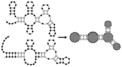
Figure 6: Grouping of two RNA structures according to their common bonds: Each pair of RNA secondary structures like the one on the left hand side can be classified according to the bonds which are common to both structures (open circles.) These common bonds form by themselves an RNA secondary structure (right hand side.) Thus, the sum over all pairs of secondary structures can be written as the sum over all possible secondary structures of the common bonds. The weight of each common bond structure is then given by the interaction energies of common bonds and the summation over all possibilities of arranging non-common bonds in the given common-bond structure. Since non-common bonds have to be compatible with the common bond structure, the latter sum factorizes into independent contributions of all the loops of the common bond structure (grey circles.) Each such contribution solely depends on the number of non-common-bond bases in each of these loops.

Note that the common bonds partition the diagram into a number of “bubbles”, shown as the shaded regions in Fig. 6. Due to the exclusion of pseudo-knots from the valid secondary structures, only bases belonging to the same bubble can be paired with each other. Thus, the two-replica partition function can be written as

$${\cal G}(N+1;\widetilde{q})=\sum_{S\in{\bf S}(N)}(q^{2}\widetilde{q})^{|S|}\prod_{\mbox{bubble $i$ of $S$}}{\cal Q}_{i}(\ell_{i}+1),$$ (29)

where the factor $q^{2}\widetilde{q}$ is the weight of each common bond, and ${\cal Q}_{i}(\ell_{i}+1)$ is the sum of all possible intra-replica pairings of of the $i^{\rm th}$ bubble of $\ell_{i}$ bases in $S$, with the restriction that there are no common bonds.

It should be clear that ${\cal Q}_{i}$ neither depends on the number of stems branching out from the bubble $i$ nor the positions of these stems relative to the bases within the bubble. It depends on $S$ only through the number of bases $\ell_{i}$ in the bubble and is given by a single function ${\cal Q}$ independent of $i$. This function can be written explicitly as

$${\cal Q}(\ell+1)\equiv\sum_{\begin{array}[]{c}S_{1},S_{2}\in{\bf S}(\ell)\\ S_{1}\cap S_{2}=\emptyset\end{array}}q^{|S_{1}|+|S_{2}|}.$$ (30)

With Eqs. (29) and (30), the two-replica problem is reduced to an effective single homogeneous RNA problem, with an effective Boltzmann weight $q^{2}\widetilde{q}$ for each pairing, and an effective weight ${\cal Q}$ for each single stranded loop. As described in Appendix A, this problem becomes formally analogous to that of an RNA in the vicinity of the denaturation transition, with ${\cal Q}$ being the weight of a single polymer loop fluctuating in $6$-dimensional embedding space. The competition between pairing energy and the bubble entropy leads to a phase transition for the two-replica problem, analogous to the denaturation transition for a single RNA.

The details of this transition are given in Appendix B, where the partition function (29) is solved exactly. The exact solution exploits the relation

$${\cal Q}(N)={\cal G}(N;\widetilde{q}=0)$$ (31)

which follows from the definitions (28) and (30), and turns Eq. (29) into a recursive equation for ${\cal G}$. The solution is of the form

$${\cal G}(N;\widetilde{q})\sim N^{-\theta}\zeta^{N}(q,\widetilde{q})$$ (32)

for large $N$, with two different forms for $\theta$ and $\zeta$ depending on whether $\widetilde{q}$ is above or below the critical value

$$\widetilde{q}_{c}=1+\frac{1}{q^{2}\sum_{N=1}^{\infty}NG^{2}(N)(1+2\sqrt{q})^{-2(N-1)}}.$$ (33)

Here $G(N)$ is the molten phase partition function, whose large $N$ asymptotics is given by Eq. (23) and whose values for small $N$ can be calculated explicitly from the recursion Eq. (18). Thus, the actual value of $\widetilde{q}_{c}$ can be found for any given $q$.

For $\widetilde{q}<\widetilde{q}_{c}$, we have $\theta=3$ and

$$\zeta=(1+2\sqrt{q})^{2}+q^{2}(\widetilde{q}-1){g_{1}}(q),$$ (34)

where

$${g_{1}}(q)=\sum_{N=1}^{\infty}G^{2}(N)(1+2\sqrt{q})^{-2N},$$ (35)

according to Eqs. (72) and (74). In this regime, the two-replica partition function ${\cal G}$ is essentially a product of two single-replica partition functions $G$. Compared to Eq. (23), we can identify $\theta$ as $2\theta_{0}$, and $\zeta$ as a modified version of $z_{0}^{2}\equiv(1+2\sqrt{q})^{2}$. Since there is no coupling of the two replicas beyond a trivial shift in the free energy per length, $f=-k_{B}T\ln\zeta$, we conclude that the disorder coupling is irrelevant. Hence the two-replica system is in the molten phase in this regime.

For $\widetilde{q}>\widetilde{q}_{c}$, we have $\theta=3/2$ and $\zeta$ is given as the implicit solution of an equation involving only single-replica partition functions as shown in Eqs. (79) and (82). Here, the partition function of the two-replica system is found to have the same form as that of the single-replica system in (23). This result implies that the two replicas are locked together via the disorder coupling, and the molten phase is no longer applicable in this regime.

Of course, as already explained above, only the weak-disorder limit (i.e., $\beta^{2}D\ll 1$) of the two-replica problem is of relevance to the full random RNA problem. In this limit, $\widetilde{q}\approx 1+\beta^{2}D$ while $\widetilde{q}_{c}$ is found by evaluating Eq. (33) with $q\approx e^{-\beta\overline{\varepsilon}}$. It can be easily verified that $\widetilde{q}_{c}>1$ as long as $q$ is finite. Thus in the weak disorder limit, we have $\widetilde{q}<\widetilde{q}_{c}$, indicating that the molten phase is an appropriate description for the random RNA. Unfortunately, the two-replica calculation cannot be used in itself to deduce whether the molten phase description breaks down at sufficiently strong disorder or low temperature. Based on this analysis, we cannot conclude whether the type of phase transition obtained for the two-replica problem is present in the full problem.

IV Effect of Sequence Randomness: Low Temperature Behavior

Having established the validity of the molten phase description of random RNA molecules at weak disorder or high temperatures, we now turn our focus onto the low temperature regime. First, we will give an analytical argument for the existence of a glass phase at low temperatures. Then, we will present extensive numerical studies confirming this result and characterizing this glass phase.

IV.1 Existence of a glass phase

We will start by showing that the molten phase cannot persist for all temperatures down to $T=0^{+}$. To this end, we will assume that long random RNA is in the molten phase for all temperatures, i.e., that the partition function for any substrand of large length $L\gg 1$ is given by

$$Z(L)=A(T)L^{-\frac{3}{2}}\exp[-\beta f_{0}(T)L]$$ (36)

with some effective temperature-dependent prefactor $A(T)$ and free energy per length $f_{0}(T)$. Then, we will show that this assumption leads to a contradiction below some temperature $T^{*}>0$. This contradiction implies that the molten phase description breaks down at some finite $T_{\mathrm{g}}\geq T^{*}$. To be specific, we will consider the sequence disorder model (2) in this analysis.

The quantity we will focus on is again the free energy $\Delta F(N)$ of the largest possible pinch. Under the assumption that the random sequences are described by the molten phase, it is given by

$$\overline{\Delta F}(N)=\frac{3}{2}k_{B}T\ln N$$ (37)

for large $N$ and all $T$ independently of the values of the effective prefactor $A(T)$ and the free energy per length $f_{0}(T)$ (see Eq. (26).)

On the other hand, we can study this pinching free energy for each given sequence of bases drawn from the ensemble of random sequences. For each such sequence, we can look for a continuous segment of $\ell\ll N$ Watson-Crick pairs $b_{i}$–$b_{j},b_{i+1}$–$b_{j-1},\ldots,b_{i+\ell-1}$–$b_{j-\ell+1}$ where the bases $b_{i}\ldots b_{i+\ell-1}$ are within the first half of the molecule and the bases $b_{j-\ell+1}\ldots b_{j}$ are in the second half (see Fig. 7(a).) For random sequences, the probability of finding such exceptional segments decreases exponentially with the length $\ell$, with the largest $\ell$ in a sequence of length $N$ being typically

$$\ell=\lambda^{-1}\ln N.$$ (38)

For exact complementary matches, the proportionality constant is known to be $\lambda=\ln 2$ arra90 .

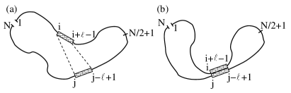
Figure 7: Finding a good match in a RNA sequence: (a) shows the position of two pieces with exactly complementary bases one of which is between positions $2$ and $N/2$ and the other of which is between positions $N/2+2$ and $N$. Such a piece of length $\ell\sim\ln N$ can be found for almost all sequences. (b) shows how restricting configurations to those in which the good match forms Watson-Crick base pairs splits the molecule into two loops which can still form base pairs within the loops independently from each other.

Now, we calculate the pinching free energy

$$\Delta F(N)=F_{\mathrm{pinched}}-F_{\mathrm{unpinched}}$$ (39)

by evaluating the two terms separately. The partition function for the unpinched sequence contains at least all the configurations in which the two complementary segments $b_{i}\ldots b_{i+\ell-1}$ and $b_{j-\ell+1}\ldots b_{j}$ are completely paired (see Fig. 7(b)). Thus,

$$F_{\mathrm{unpinched}}\leq F_{\mathrm{paired}}$$ (40)

where $F_{\mathrm{paired}}$ is the free energy of the ensemble of structures in which the two complementary segments are paired. The latter is the sum of the free energy of the paired segments and those of the two remaining substrands $b_{i+\ell}\ldots b_{j-\ell}$ of length $L_{1}\!=\!j\!-\!i\!-\!2\ell\!+\!1$ and $b_{j+1}\ldots b_{i-1}$ (wrapping around the end of the molecule) of length $L_{2}\!=\!N\!+\!i\!-\!j\!-\!1$, i.e.,

$$F_{\mathrm{paired}}\!\!=\!\!-\ell u_{\mathrm{m}}\!+(N\!-\!2\ell)f_{0}+{\textstyle\frac{3}{2}}k_{B}T\big{[}\!\ln(L_{1})\!+\!\ln(L_{2})\big{]}.$$ (41)

The free energy $F_{\mathrm{pinched}}$ in the presence of the pinch is, by the assumption of the molten phase, the interaction energy of the pinched base pair $b_{1}$–$b_{N/2+1}$ plus the molten free energy of the substrand $b_{2}\ldots b_{N/2}$ and the molten free energy of the substrand $b_{N/2+2}\ldots b_{N}$, i.e., according to Eq. (36)

$$F_{\mathrm{pinched}}=f_{0}(T)N+2\times\frac{3}{2}k_{B}T\ln N$$ (42)

up to terms independent of $N$. Combining this with Eqs. (39), (40), and (41), we get

$$\Delta F(N)\!\geq\!\frac{3}{2}k_{B}T[2\ln N\!-\!\ln L_{1}\!-\!\ln L_{2}]+\ell[u_{\mathrm{m}}\!+\!2f_{0}(T)].$$ (43)

Using the result (38) and that $L_{1}$ and $L_{2}$ are typically proportional to $N$, we finally obtain

$$\overline{\Delta F}(N)\geq[u_{\mathrm{m}}+2f_{0}(T)]\lambda^{-1}\ln N$$ (44)

for large $N$. This is only consistent with Eq. (37) if

$$\frac{3}{2}k_{B}T\geq\lambda^{-1}[u_{\mathrm{m}}+2f_{0}(T)].$$ (45)

Now, $f_{0}(T)$ is a free energy and is hence a monotonically decreasing function of the temperature. Thus the validity of the inequality (37) depends on the behavior of its right hand side at low temperatures. As $T\to 0$, the inequality can only hold if $\sigma\equiv u_{\mathrm{m}}+2f_{0}(T=0)\leq 0$. Since the average total energy at $T=0$ is $u_{\mathrm{m}}$ times the average total number of matched pairs of a random sequence, then $2f_{0}(0)$ is simply the fraction of matches and $\sigma$ is the fraction of bases not matched (for $u_{\mathrm{m}}=1$.) Clearly, $\sigma$ cannot be negative, and the inequality (37) must fail at some finite temperature unless $\sigma=0$.

We can make a simple combinatorial argument to show that in most cases the fraction $\sigma$ of unbound bases must strictly be positive. To illustrate this, let us generalize the “alphabet size” of the sequence disorder model of Sec. II.1.2 from $4$ to an arbitrary even integer $K\geq 2$. We will still adopt the energy rule (2) where each of the $K$ bases can form a “Watson-Crick” pair exclusively with one other base. Let us estimate the number of possible sequences for which the fraction of unmatched bases $\sigma$ is zero in the limit of long sequence length $N$ at $T=0$. Since at $T=0$, only Watson-Crick (W-C) pairs can be formed, we only need to count the number of sequences for which the fraction of W-C paired bases is $1$. This means that except for a sub-extensive number of bases, all have to be W-C paired to each other. From the mountain picture (Fig. 3), it is clear that the number of possible secondary structures for such sequences must scale like $2^{N}$, since the fraction of horizontal steps is non-extensive so that at each step, there are only the possibilities for the mountain to go up or down. For each of the $N/2$ pairings in one of these $2^{N}$ structures, there are $K$ ways of choosing the bases to satisfy the pairing. So for each structure, there are $K^{N/2}$ ways of choosing the sequence that would guarantee the structure. Since there are a total of $K^{N}$ sequences, it is clear that the fraction of sequences with all (but a sub-extensive number of) W-C pairs becomes negligible if

$$(2\sqrt{K})^{N}<K^{N}.$$ (46)

Thus, for $K\geq 6$, we must have $\sigma>0$.

For $K=2$, the left hand side of Eq. (46) grows faster than its right hand side. This reflects the absence of frustration in this simple two-letter model as already discussed at the end of Sec. II.1.2. One way to retain frustration is to introduce additional constraints, e.g., the minimal hairpin length used in Ref. pagn00 . With this constraint, a structure with a sub-extensive number of unmatched bases can only contain a sub-extensive number of hairpins. In the mountain picture, this means that except for a sub-extensive number of steps, there is only one choice to go up or down at every step. This changes Eq. (46) to $K^{N/2}<K^{N}$. It ensures frustration since $\sigma>0$ for all $K$. Since a minimal length of $3$ bases is necessary in the formation of a real hairpin, real RNA is certainly frustrated by this argument. The random sequence model which we study in this paper is marginal since $K=4$ and there is no constraint on the minimal hairpin length. In this case, all the prefactors on the two sides of Eq. (46) (e.g., the overcounting of sequences that support more than one structure) must be taken into account. We will not undertake this effort here, but will verify numerically in Sec. IV.3 that $\sigma>0$ also in this case.

In all cases with $\sigma>0$, it follows that there is some unique temperature $T^{*}$ below which the consistency condition (45) breaks down, implying the inconsistency of the molten phase assumption in this regime. From this we conclude that there must be a phase transition away from the molten phase at some critical temperature $T_{\mathrm{g}}\!\geq\!T^{*}\!>\!0$. The precise value of the bound $T^{*}$ depends on $\lambda$ which in turn depends on the stringency of the condition we impose on the rare matching segments. For instance, if we relax the condition of exact complementarity between two segments to allow for matches within each segment, then the constant $\lambda$ will be reduced from $\ln 2$ and the value of $T^{*}$ will increase. This will be discussed more in Sec. IV.3.

IV.2 Characterization of the glass phase

The above argument does not provide any guidance on the properties of the low temperature phase itself. In order to characterize the statistics of secondary structures formed at low temperatures, we re-do the simulations reported in Sec. III.1 at $k_{B}T=0.025$ in energy units set by $u_{\mathrm{m}}=u_{\mathrm{mm}}=1$. At this temperature, an unbound base pair is penalized with a factor $e^{40}$ relative to a Watson-Crick base pair, and a non Watson-Crick base pair is penalized even more. Thus, only the minimal energy structures contribute (for the sequence lengths under consideration here), and we may regard this effectively as at $T=0$. As in Sec. III.1, we average over $10,000$ realizations of the disorder for $N\in\{10,20,40,80,160,320\}$, over $2,000$ realizations for $N=640$ and over $1,000$ realizations for $N\in\{1280,2560\}$.

Fig. 8 shows the results for the ladder size $\langle h\rangle$ of the structures for the three models of disorders. The ladder size still scales algebraically with the length of the sequences, with numerically determined exponents ranging from $\overline{\langle h\rangle}\sim N^{0.65}$ to $\overline{\langle h\rangle}\sim N^{0.69}$ for the different choices of disorder. They are clearly different from the square root behavior (dotted line) expected of the molten phase. Thus this result reaffirms our expectation that the secondary structures of a random RNA sequence at zero temperature indeed belongs to a phase that is different from the molten phase.

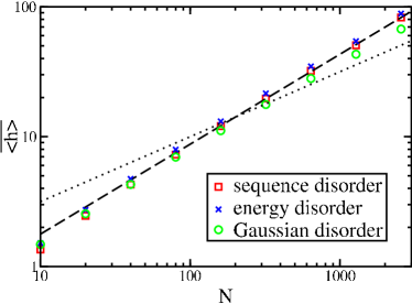
Figure 8: Scaling of the average size $\overline{\langle h\rangle}$ of secondary structures in the low temperature phase with the length $N$ of the sequences: The plot shows data for three different choices of disorder according to Eqs. (2), (4), and (5) at $T=0.025$. The average system size follows a power law. However, the best fit of the data for sequence disorder at $N\geq 160$ to a power law indicated by the dashed line leads to an exponent of $\overline{\langle h\rangle}\sim N^{0.69}$. The corresponding fits for energy and Gaussian disorder yield exponents of $\overline{\langle h\rangle}\sim N^{0.69}$ and $\overline{\langle h\rangle}\sim N^{0.65}$, respectively. This is distinctively different from the square root behavior of the molten phase indicated by the dotted line. The comparison of this plot with its counterpart in Fig. 5(a) suggests that the behavior of RNA secondary structures at low temperatures is different from the molten phase.

IV.2.1 A criterion for glassiness

A key question in characterizing the thermodynamic properties of disordered systems is whether the zero-temperature behavior persists for a range of finite temperatures. If it does, then the system is said to have a finite-temperature glass phase. One way to address this question is to study the overlap between different replicas of the RNA molecule as mentioned earlier. If a non-trivial distribution of these overlaps with significant weight on large overlaps persists into finite temperatures, then the finite-temperature glass phase exists. This approach was taken by previous numerical studies higg96 ; pagn00 ; hart01 ; pagn01 . Unfortunately, the results are inconclusive and even contradictory due to the weakness of the proposed phase transition — only the fourth temperature derivative of the free energy seems to show an appreciable singularity. Moreover, due to limitations in the sequence lengths probed, it was difficult to get a good estimate of the asymptotic behavior of the overlap distribution.

In our study, we adopt a different approach based on the droplet theory of Fisher and Huse huse91 . In this approach, one studies the “large scale low energy excitations” about the ground state. This is usually accomplished by imposing a deformation over a length scale $\ell\gg 1$ and monitoring the minimal (free) energy cost of the deformation. This cost is expected to scale as $\ell^{\omega}$ for large $\ell$. A positive exponent $\omega$ indicates that the deformation cost grows with the size. If this is the case, the thermodynamics is dominated by a few low (free) energy configurations in the thermodynamic limit, and the statistics of the zero-temperature behavior persists into finite temperatures. On the other hand, if the exponent $\omega$ is negative, then there are a large number of configurations which have low overlap with the ground state but whose energies are similar to the ground state energy in the thermodynamic limit. At any finite temperature $T$, a finite fraction of these configurations (i.e., those within $O(k_{B}T)$ of the ground state energy) will contribute to the thermodynamics of the system. The zero temperature behavior is clearly not stable to thermal fluctuations in this case, and no thermodynamic glass phase can exist at any finite temperature. The analysis of the previous section indicate the existence of a glass phase; thus we expect to find the excitation energy to increase with the deformation size.

It should be noted that this criterion for glassiness is purely thermodynamical in nature and does not make any statement about kinetics. A system which is not glassy thermodynamically can still exhibit very large barriers between the many practically degenerate low energy configurations, leading to a kinetic glass. A study of the kinetics of RNA, e.g., in terms of barrier heights, is naturally dependent on the choice of allowed dynamical pathways to transform one RNA secondary structure into another one morg96 ; morg98 ; flam00 ; isam00 . Since the latter is a highly non-trivial problem, we will restrict ourselves to thermodynamics and use the droplet picture explained above as our criterion for the existence of a glass phase.

IV.2.2 Droplet excitations

According to the criterion for glassiness just presented, our goal is to determine the value of the exponent $\omega$ for random RNAs numerically. To this end, the choice of “large scale low energy excitations” needs some careful thoughts. As in every disordered system, there is a very large number of structures which differ from the minimal energy structure only by a few base pairs and which have an energy only slightly higher than the minimum energy structure. These structures are clearly not of interest here. Instead we need to find a controlled way of generating droplet excitations of various sizes.

We propose to use the pinching method introduced in Sec. II.1.4 as a way to generate the deformation, and regard the difference between the minimal energy pinched structure and the ground state structure as the droplet excitation. There are several desirable features about these pinch-induced deformations: First, it gives a convenient way of controlling the size of the deformation. If $(i,i^{\prime})$ is a base pair that is bound anyways in the ground state, pinching this base pair does not have any effect and $\Delta F_{i,i^{\prime}}=0$. If we pinch base $i$ with some other base $j\not=i^{\prime}$, then we force at least a partial deformation of the ground state, for bases in the vicinity of $i$, $i^{\prime}$, and $j$. This is illustrated in Fig. 9 with the deformed region indicated by the shade. As we move the pinch further away from the ground state pairing, we systematically probe the effect of larger and larger deformations (provided that a pinch only induces local deformation as we will show). Second, the minimal energy or the free energy of the secondary structures subject to the pinch constraint is easily calculable numerically by the dynamic programming algorithm as shown in Eqs. (10) and (11). Third, the pinching of the bases in a sense mimics the actual dynamics of the RNA molecule at low temperatures. In order for the molecule to transform from one secondary structure to another at a temperature where all matching bases should be paired, the bases have to make local rearrangements of the secondary structures much like the way depicted in Fig. 9 flam00 . Thus, the pinching energy provides the scale of variation in the local energy landscape for such rearrangements. Finally, “pinching” of a real RNA molecule can be realized in the pulling of a long molecule through a pore gerl02 .

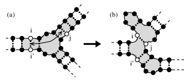
Figure 9: Deformation of a minimal energy structure by pinching: The two bases $i$ and $i^{\prime}$ (open circles) form a base pair in the indicated minimal energy structure (a). Thus, forcing these two bases to be bound by pinching does not affect the structure at all. Pinching of $(i,j)$ on the other hand will lead to a local rearrangement (shaded region) of the structure as shown in (b). The effect of such a pinch depends on the number of base pairs of the minimal energy structure the pinch is incompatible with. As indicated by the arrow in (a), this number is given by the ladder distance $h_{i,j}$ between $i$ and $j$; in this example $h_{i,j}=3$.

A key question to the utility of these pinch deformations is whether the deformation is confined to the local region of the pinch as depicted in Fig. 9 or whether it involves a global rearrangement of the structure. To test this aspect, we numerically study the changes in pinch free energy as a function of the “size” of a pinch. Here, the definition of the pinch size needs some thought. Consider a specific sequence whose minimal energy structure is $S^{*}$. If the binding partner of base $i$ is base $i^{\prime}$ in the minimal energy structure, a natural measure for the size of a pinch $(i,j)\notin S^{*}$ with $i<j<i^{\prime}$ would be the ladder distance $h_{i,j}$ between base $i$ and base $j$; see Fig. 9. From the mountain representation (Fig. 3(b)), it is easy to see that this is just the difference of the respective ladder distances of base $j$ and base $i$ from base $1$ as defined in Eq. (13), i.e., $h_{i,j}=h_{j}(S^{*})-h_{i}(S^{*})$. To find how the excitation energy depend on the pinch size, we just need to follow how the pinching free energy $\Delta F_{i,j}$’s depend statistically on the size $h_{i,j}$’s. To do so, we choose a large number of random sequences, and determine the minimal energy structure $S^{*}$ for each of these sequences. Then, we compute the pinch free energies $\Delta F_{i,j}$ and the pinch size $h_{i,j}$ for all possible pinches $(i,j)$ for each sequence. Afterwards, we average over all $\Delta F_{i,j}$’s with the same pinch size $h_{i,j}$ over all of the generated random sequences to obtain the function

$$\overline{{\delta F}}(\delta h)\equiv\sum_{i,j}\overline{\Delta F_{i,j}\,\delta_{\delta h,h_{i,j}}}\Bigg{/}\sum_{i,j}\overline{\delta_{\delta h,h_{i,j}}}.$$ (47)

The results obtained at $k_{B}T=0.025$ for a large range of sequence sizes from $N=80$ to $N=2,560$ are shown in Fig. 10(a). We see that the data for different $N$’s fall on top of each other for small $\delta h$’s, with

$$\overline{\delta F}\sim(\delta h)^{0.27}.$$ (48)

This behavior explicitly shows that the pinch deformation is a local deformation. In particular, we see that for small $\delta h$’s, the free energy cost is independent of the overall length $N$ of the molecule.

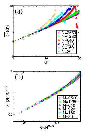
Figure 10: Pinching free energy as a function of the number $\delta h$ of minimal energy structure base pairs that are incompatible with the pinch for random sequence disorder at $T=0.025$: (a) shows the raw data. For small $\delta h$ the pinching free is independent of the length $N$ of the molecule and obeys a power law $\overline{\delta F}(\delta h)\sim(\delta h)^{0.27}$ (dashed line.) This is consistent with the expectation that pinching at small $\delta h$ leads to local rearrangements of the secondary structure. The apparent non-monotonic behavior at large $\delta h$ is due to the small number of sequences in which such a value of $\delta h$ is realized. (b) shows the same data, but the scaling of $\delta h$ with $N$ is chosen in accordance with Fig. 8 while the scaling of the pinching free energy is chosen in accordance with the power law dependence estimated above.

It is interesting to see at which $\delta h$ the entire sequence is involved. One expects $\delta h_{\rm max}\sim\langle h\rangle\sim N^{0.69}$ since $\langle h\rangle$ gives the typical scale of the maximum ladder length. To test this, we normalized $\delta h$ by $N^{0.69}$ and $\overline{\delta F}$ by $N^{0.19}$ (such that the relation (48) is preserved for small $\delta h$’s). The result is shown in Fig. 10(b). We see that the data is approximately collapsed onto a single curve, indicating that pinching is indeed a good way of imposing a controlled deformation from the ground state.

IV.2.3 A marginal glass phase

The scaling plot of Fig. 10(b) indicates strongly that the energy associated with the pinch deformation increases with the size of the deformation, i.e., $\overline{\delta F}\sim(\delta h)^{0.27}\sim N^{0.19}$. However, the effective exponent involved is small, making the result very susceptible to finite size effects. In order to decide on the glassiness of the system, we want to focus on the energy scales associated with the largest pinch deformations from the ground state. Assuming that there is only a single energy scale associated with large pinches, we again study the free energy $\Delta F(N)$ of the largest pinch as defined in Eq. (12) and average this over the ensemble of sequences.

The results are shown in Fig. 11(a) for the three models of disorders. Although a weak power law dependence of $\overline{\Delta F}(N)$ on $N$ cannot be excluded, the fitted exponents obtained for the three models are different from each other, ranging from $0.09$ to $0.19$. This is a strong sign of concern, since the exponents are expected to be independent of details of the models. In Fig. 11(b), the same data is plotted on a log-linear scale. The data fall reasonably on a straight line for each of the models (especially for large $N$’s), suggesting that the pinching free energy may actually increase logarithmically with the sequence length, similar to what is expected of the behavior in the molten phase ! However in this case, the prefactor of the logarithm depends on the choice of the model and is much larger than the factor $\frac{3}{2}k_{B}T$ expected of the molten phase; see Eq. (26). For example, for the numerical data obtained at $k_{B}T=0.025$, the prefactor is approximately $0.9$ for the sequence disorder model, while the expected slope for the molten phase is $0.0375$ at this temperature. Having different logarithmic prefactors for the different models is not a concern, since a prefactor is a non universal quantity. Thus, our numerical results favor a logarithmically increasing pinch energy, with a prefactor much exceeding $k_{B}T$ at low temperature.

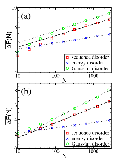
Figure 11: Pinching free energies at low temperature: (a) shows a double logarithmic plot with fits to power laws for the data with $N\geq 160$. The exponents are $N^{0.18}$, $N^{0.09}$, and $N^{0.19}$ for the sequence, energy, and Gaussian disorder respectively. (a) shows the same data in a single logarithmic plot together with the best fits to a logarithmic dependence on $N$. The statistical error of the data points is about the size of the symbols for large $N$ and smaller than that for $N\leq 640$. Due to the apparent systematic bending of the data in the double logarithmic plot (b) we conclude that a logarithmic dependence fits the data better although we cannot exclude a power law behavior with a very small power.

What does this tell us about the possible glass phase of the random RNA? In order to answer this question, we should remind ourselves that rather special deformations are chosen in this study. For our choice of pinch deformations, we observe a logarithmic dependence of the gap between the ground state energy and the energy of the excited configurations on the length of the sequence or deformation. This corresponds to the marginal case of the droplet theory where the exponent $\omega$ vanishes. Since the pinching free energies are increasing with length, we cannot exclude a glass phase in the case $\omega=0$. We can say, though, that the increase of the excitation energy with length is at most a power law with a very small exponent and most probably even less than any power law. Therefore, a possible glass phase of RNA has to be very weak. If it turns out that the excitation energy is indeed a logarithmic function of length, with a non-vanishing prefactor as $T\to 0$ as our numerics suggest, then the low-temperature phase would be categorized formally as a marginal glass phase, analogous to behaviors found in some well-studied model of statistical mechanics card82 ; kors93 ; hwa94 . In any case, we should note that the actual difference in the excitation energy is only a factor of $4$ across two-and-a-half decades in length. Thus the glassy effect will be weak for practical purposes. On the other hand, the weak dependence of the excitation energy on length may be the underlying cause of discrepancies in the literature pagn00 ; hart01 ; pagn01 regarding the existence of the glass phase for the random RNA.

IV.3 Estimation of the phase transition temperature

Now that we have studied in great detail the behavior of random RNA in the low and the high temperature phase, we describe its behavior at intermediate temperatures. To this end, we again study the pinch free energies $\overline{\Delta F}(N)$ defined in Eq. (12), but this time over a large range of temperatures. We concentrate on the sequence disorder model Eq. (2) with $u_{\mathrm{m}}=u_{\mathrm{mm}}=1$, and study sequences of lengths up to $N=1,280$.

From Secs. II.2.3, III.1, and IV.2.3, we know that the pinch free energy $\overline{\Delta F}(N)$ depends logarithmically on the sequence length $N$ at both low and high temperatures. Indeed, this logarithmic behavior seems to hold for all temperatures studied. The data for each temperature can easily be fitted to the form

$$\overline{\Delta F}(N)=a(T)\ln N+c(T)$$ (49)

The prefactor $a(T)$ is found to depend on temperature in a non-monotonic way as shown in Fig. 12. The figure contains values of $a(T)$ extracted by fitting the data for $N\geq 160$ to the form Eq. (49). The uncertainty of this fit is on the order of the size of the symbols or smaller. For high temperatures, we find $a(T)\approx\frac{3}{2}k_{B}T$ (dashed line in Fig. 12) as expected for the molten phase. At low temperatures, it starts from a finite value of the order $1$ and decreases linearly with temperature, as $a(T)\approx 0.97-2.7k_{B}T$ (dotted line in Fig. 12). If we identify the glass transition temperature $T_{g}$ as the intersection of the dashed and the dotted lines, we get

$$k_{B}T_{\mathrm{g}}\approx 0.25.$$ (50)

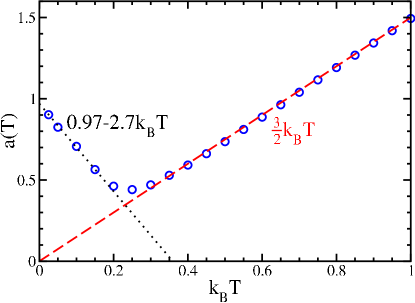
Figure 12: Prefactor $a(T)$ of the logarithmic dependence of $\overline{\Delta F}$ on $N$ for random RNA sequences generated by the sequence disorder model: At high temperatures, the prefactor indicated by the circle is well-described by the dashed line $\frac{3}{2}k_{B}T$ expected of the molten phase. At low temperatures, it again has a linear temperature dependence and is empirically fitted by the dotted line, $0.97-2.7k_{B}T$. The numerical uncertainty in $a(T)$ is of the order of or smaller than the size of the symbols.

It is interesting to compare this estimate with the lower bound $T^{*}$ for the glass transition temperature given in Sec. IV.1. According to the consistency condition (45), this lower bound is defined by

$$\lambda^{-1}[u_{\mathrm{m}}+2f_{0}(T^{*})]=\frac{3}{2}k_{B}T^{*}$$ (51)

with $\lambda=\ln 2$. It is necessary to determine the temperature dependence of the quantity $u_{\mathrm{m}}+2f_{0}(T)$ on the left hand side of this equation numerically. To do this, we measure the total free energy of each sequence generated. Averaging these free energies over all the sequences of a given length $N$ and temperature $T$, and dividing the results by the respective lengths $N$, we obtain an estimate $f_{0}(T;N)$ of the free energy per length which approaches the desired $f_{0}(T)$ for large $N$.

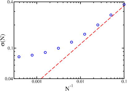
Figure 13: Sequence length dependence of the fraction of unbound bases $\sigma(N)=u_{\mathrm{m}}+2f_{0}(T\approx 0;N)$: The data shown is taken at $k_{B}T=0.025$. For small $N$ it is dominated by the statistical fluctuations in the number of bases according to Eq. (52) (the dashed line). At large $N$, it saturates to a positive constant.

Fig. 13 shows how these estimates depend on the sequence length $N$ for the lowest temperature $k_{B}T=0.025$ studied. Instead of the free energy per length itself, the figure shows the fraction of unbound bases $\sigma(N)=u_{\mathrm{m}}+2f_{0}(T\approx 0;N)$. For short sequences these estimates show a clear dependence on the sequence length $N$. This can be understood in terms of sequence-to-sequence fluctuations in the maximum number of possible pairings, due to fluctuations in the actual number of each type of bases present in a given sequence, even if all four bases are drawn with equal probability. This effect can be quantified by assuming that there is no frustration for small $N$, i.e., for any given sequence of the four bases $A$, $C$, $G$, and $U$, a secondary structure with the maximal number of Watson-Crick base pairs can be formed. If we denote by $n_{X}$ the number of times that the base $X$ appears in the sequence, the maximal number $M$ of pairings is given by $M=\min\{n_{A},n_{U}\}+\min\{n_{G},n_{C}\}$. The fraction of unbound bases $1-2M/N$ due to this effect can be computed straightforwardly approximating the multinomial distribution of $n_{A}-n_{U}$ by an appropriate Gaussian distribution, with the result

$$1-\frac{2M}{N}\approx 2/\sqrt{\pi N}.$$ (52)

We expect this effect to be responsible for the increase in $\sigma(N)$ found in Fig. 13. Indeed this effect, as indicated by the dashed line in the figure, explains the $N$ dependence of $\sigma(N)$ well for $N<100$. However, we also see from the figure a clear saturation effect at large $N$. This saturation reflects the finite fraction of unbound bases which is a frustration effect forced upon the system through the restriction on the type of allowed pairings in a allowed secondary structure. The unbound fraction $\sigma\approx 0.08$ is finite asymptotically as expected in Sec. IV.1. Note that this value is remarkably small, as it implies that in the ground state structure of our toy random sequence, more than $90\%$ of the maximally possible base pairs are formed. But this is an artifact of the very simple energy rule used in our toy model. This fraction certainly will become smaller if the realistic energy rules are used, making the system more frustrated hence more glassy.

In order to obtain the temperature dependence of the quantity $u_{\mathrm{m}}+2f_{0}(T)$ on the left hand side of Eq. (51), we will use its value at $N=1,280$ as an estimate of its asymptotic value. The results are shown in Fig. 14. The behavior at low temperatures can be described by a linearly decreasing function, shown as the dotted line in Fig. 14. According to Eq. (51), the temperature $T^{*}$ is obtained as the intersection of this curve and $\frac{3}{2}\lambda k_{B}T$, shown as the dashed line in Fig. 14 for $\lambda=\ln 2$. We find

$$k_{B}T^{*}\approx 0.066$$ (53)

which is consistent with the estimate (50), but is a rather weak bound. Improved bounds on $T_{\mathrm{g}}$ can be made by relaxing the condition of perfect complementarity of the two segments imposed in Sec. IV.1. This leads to larger values of the prefactor $\lambda^{-1}$ in Eq. (51), hence a smaller slope for the dashed line in Fig. 14, and a larger value of $T^{*}$. While the details of improved bounds will be discussed elsewhere, let us remark here that from Fig. 14 it is clear that no matter what the slope of the dashed line becomes, we will never have $T^{*}$ larger than the temperature of $k_{B}T\approx 0.22$ where the quantity $u_{\mathrm{m}}+2f_{0}(T)$ goes below zero. Thus, these estimates will always be consistent with the observed glass transition temperature of $k_{B}T_{g}\approx 0.25$.

Moreover, we note that the low temperature behavior $u_{\mathrm{m}}+2f_{0}(T)\approx 0.089-0.31k_{B}T$ as indicated by the dotted line in Fig. 14, appears to be roughly related to the behavior of $a(T)$ (dotted line in Fig. 12) in the same temperature range, by a single scaling factor of approximately $0.1$. Thus, it is possible that

$$a(T)\approx\lambda^{-1}[u_{\mathrm{m}}+2f_{0}(T)]$$ (54)

if it turns out that $\lambda^{-1}\approx 0.1$ for $T<T_{g}$. If this is the case, then it means the procedure we used to estimate the pinch energy in Sec. IV.1 is quantitatively correct, implying that the ground state of a random RNA sequence indeed consists of the matching of rare segments independently at each length scale. It will be useful to pursue this analysis further using a renormalization group approach similar to what was developed for the denaturation of heterogeneous DNAs by Tang and Chaté tang00 .

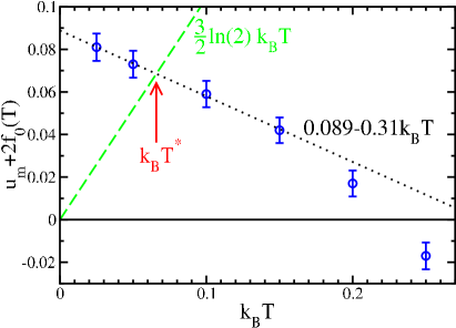
Figure 14: Estimation of $T^{*}$: The symbols show numerical estimates of the quantity $u_{\mathrm{m}}+2f_{0}(T)$ for different temperatures. The estimates are obtained by averaging the numerically determined free energy of $1,000$ random sequences of length $N=1,280$ generated by the sequence disorder model Eq. (2) with $u_{\mathrm{m}}=u_{\mathrm{mm}}=1$. The low temperature behavior can be described reasonably well by the expression $0.089-0.31k_{B}T$ (dotted line). The consistency condition (45) for the molten phase breaks down when this line intersects $\frac{3}{2}\ln(2)k_{B}T$ (the dashed line). This yields $k_{B}T^{*}\approx 0.066$ as a lower bound for the glass transition temperature of this system.

V Summary and Outlook

In this manuscript, we studied the statistical properties of random RNA sequences far below the denaturation transition so that bases predominantly form base pairs. We introduced several toy energy models which allowed us to perform detailed analytical and numerical studies. Through a two-replica calculation, we show that sequence disorder is perturbatively irrelevant, i.e., an RNA molecule with weak sequence disorder is in a molten phase where many secondary structures with comparable total energy coexist. A numerical study of the model at high temperature recovers scaling behaviors characteristic of the molten phase. At very low temperatures, a scaling argument based on the extremal statistics of rare matches suggest the existence of a different phase. This is supported by extensive numerical results: Forced deformations are introduced by pinching distant monomers along the backbone; the resulting excitation energies are found to grow very slowly (i.e., logarithmically) with the deformation size. It is likely that the low temperature phase is a marginal glass phase. The intermediate temperature range is also studied numerically. The transition between the low temperature glass phase and the high temperature molten phase is revealed by a change in the coefficient of the logarithmic excitation energy, from being disorder dominated to entropy dominated.

From a theoretical perspective, it would be desirable to find an analytical characterization of the low temperature phase. If the excitation energy indeed diverges only logarithmically, one has the hope that this may be possible, e.g., via the replica theory, as was done for another well known model of statistical physics kors93 . It should also be interesting to include the spatial degrees of freedom of the polymer backbone (via the logarithmic loop energy), to see how sequence disorder affects the denaturation transition. Another direction is to include sequence design which biases a specific secondary structure, e.g., a stem-loop bund99 . From a numerical point of view, it is necessary to perform simulations with realistic energy parameters to assess the relevant temperature regimes and length scales where the glassy effect takes hold. To make potential contact with biology, one needs to find out whether a molten phase indeed exists between the high temperature denatured phase and the low temperature glass phase for a real random RNA molecule, and which phase the molecule is in under normal physiological condition. Finally, it will be very important to perform kinetic studies to explore the dynamical aspects of the glass phase. Despite the apparent weakness of the thermodynamic glassiness, the kinetics at biologically relevant temperatures is expected to be very slow for random sequences isam01 .

Appendix A Heuristic derivation of the two-replica phase transition

Before we describe the exact solution for the two-replica problem, as defined by the partition function ${\cal G}$ in Eq. (29) and the bubble weight ${\cal Q}$ in Eq. (30), we first provide here a heuristic derivation of the qualitative results. This mainly serves to give a flavor of the two-replica problem in the language of theoretical physics.

To this end, we define the quantity $\Pi(N)$ to be the partition function over all two replica configurations of a sequence of length $N-1$ under the constraint that base $1$ and base $N-1$ form a common bond. It is easy to see that

$$\Pi(N)=\widehat{q}\,{\cal G}(N-2;\widetilde{q})$$ (55)

where we set

$$\widehat{q}\equiv q^{2}\widetilde{q}.$$ (56)

Thus, the critical behavior of ${\cal G}(N;\widetilde{q})$ is identical to the critical behavior of $\Pi(N)$ which we will study in the following.

Due to the no pseudo knot constraint of the secondary structures, $\Pi(N)$ has a very simple structure,

$$\Pi(N\!+\!1)=\widehat{q}{\cal Q}(N\!-\!1)$$

$$+\!\!\!\!\sum_{\ell_{1},\ell_{2},n_{1}}\!\!\!\widehat{q}{\cal Q}(\ell_{1}\!+\!\ell_{2}\!+\!1)\Pi(n_{1}\!+\!1)\delta_{\ell_{1}+\ell_{2}+n_{1},N-2}$$

$$+\!\!\!\!\sum_{\ell_{1},\ell_{2},\ell_{3},n_{1},n_{2}}\!\!\!\!\!\!\!\widehat{q}{\cal Q}(\ell_{1}\!+\!\ell_{2}\!+\!\ell_{3}\!+\!1)\Pi(n_{1}\!+\!1)\times$$

$$\qquad\qquad\times\Pi(n_{2}\!+\!1)\delta_{\ell_{1}+\ell_{2}+\ell_{3}+n_{1}+n_{2},N-2}\!+\ldots$$

as illustrated in Fig. 15.

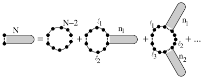
Figure 15: Recursion equation for the restricted partition function $\Pi(N+1)$: While the first and last of the $N$ bases described by $\Pi(N+1)$ always form a base pair this outermost base pair can be followed by a loop with $0,1,2,\ldots$ outgoing stems. Each of the stems is described by $\Pi$ itself while the loop is characterized by its total length that can be split into the different pieces $\ell_{i}$ in different ways.

To simplify the above equation, it is useful to introduce the $z$-transforms

$$\widehat{\Pi}[\mu] = \sum_{N=1}^{\infty}\Pi(N)e^{-\mu N}$$

$$\widehat{{\cal Q}}[y] = \sum_{N=1}^{\infty}{\cal Q}(N)e^{-yN}$$

of $\Pi$ and ${\cal Q}$. Now applying the $z$-transform to both sides of Eq. (A), we obtain

$$\widehat{\Pi}[\mu]e^{2\mu}\!\!\! = \!\!\!\widehat{q}\!\!\int\!\!\frac{\mathrm{d}y}{2\pi i}\widehat{{\cal Q}}[y]\widehat{{\cal K}}[y,\mu]\Big{[}1\!+\!\widehat{{\cal K}}[y,\mu]\widehat{\Pi}[\mu]e^{2\mu}e^{-y}$$

$$\hskip 71.13188pt+\!\left(\widehat{{\cal K}}[y,\mu]\widehat{\Pi}[\mu]e^{2\mu}e^{-y}\right)^{2}\!\!\!\!+\ldots\Big{]}$$

where

$$\widehat{{\cal K}}[y,\mu]=\frac{1}{e^{-y+\mu}-1},$$ (59)

and the inverse transform ${\cal Q}(\ell)=\int\frac{\mathrm{d}y}{2\pi i}\widehat{{\cal Q}}[y]e^{y\ell}$ was used.

Eq. (A) can be simplified greatly to the following form,

$$\widehat{\Pi}[\mu]e^{2\mu}=\widehat{q}\cdot\int\frac{\mathrm{d}y}{2\pi i}\frac{\widehat{{\cal Q}}[y]}{\widehat{{\cal K}}^{-1}[y,\mu]-\widehat{\Pi}[\mu]e^{2\mu}e^{-y}}.$$ (60)

This is reminiscent of the well-known Hartree solution to the $\phi^{4}$-theory, or equivalently the self-consistent treatment of the self-interacting polymer problem zinn89 , if we identify $\widehat{q}$ as the interaction parameter, $\widehat{{\cal K}}[y,\mu]$ as the “propagator”. The usual form of the Hartree equation

$$\widehat{\Pi}[\mu]=\widehat{q}\cdot\int\frac{\mathrm{d}^{d}k}{(2\pi)^{d}}\,\frac{1}{k^{2}+\mu-\widehat{\Pi}[\mu]}$$ (61)

corresponds to the small-$y$, small-$\mu$ limit of Eq. (60), with $-y$ playing the role of the square of the “wave number” $k$. Note that $\widehat{{\cal Q}}[y]$ plays the role of the density of (spatial) states, i.e. $dy\widehat{{\cal Q}}[y]=\frac{\mathrm{d}^{d}k}{(2\pi)^{d}}$, where $d$ denotes the dimensionality of the “embedding space”.

In the context of RNA, de Gennes used this approach to describe the denaturation of uniformly attracting RNA more than 30 years ago dege68 . Recently, this approach has been extended by Moroz and Hwa to study the phase diagram of RNA structure formation moro01 . The analysis of a self-consistent equation of the type (60) is well known moro01 ; zinn89 . The analytical properties of $\widehat{\Pi}[\mu]$ depend crucially on the form of $\widehat{{\cal Q}}[y]$. Let the singular part of $\widehat{{\cal Q}}$ be

$$\widehat{{\cal Q}}_{\mathrm{sing}}\propto(y-y_{\mathrm{c}})^{\alpha-1}$$ (62)

where $y_{\mathrm{c}}$ is the position of the singularity of $\widehat{{\cal Q}}[y]$. [Note that $\alpha=d/2$ by comparing the forms of the Hartree equations (60) and (61).] For $1<\alpha<2$, there is only one solution for all $\widehat{q}>0$, with a square root singularity in $\widehat{\Pi}[\mu]$ at some finite value of $\mu$. For $\alpha>2$, there are two possible solutions depending on the value of $\widehat{q}$. The square-root singularity exists for $\widehat{q}$ exceeding some critical value $\widehat{q}_{\mathrm{c}}(q)>0$, while for $\widehat{q}<\widehat{q}_{\mathrm{c}}(q)$, the square-root singularity disappears and $\widehat{\Pi}[\mu]$ is governed by the singularity of $\widehat{{\cal Q}}$ given in Eq. (62). Performing the inverse transform and using Eq. (55), we get ${\cal G}(N;\widetilde{q})\sim N^{-\widehat{\theta}}\zeta^{N}$ where $\zeta$ is a non-universal parameter given by the location of the singularity, while the exponent $\widehat{\theta}$ characterizes the phase of the system and is given by the singularity of $\widehat{\Pi}[\mu]$: We have $\widehat{\theta}=3/2$ if $\widehat{\Pi}[\mu]$ is dominated by the square-root singularity and $\widehat{\theta}=\alpha$ if $\widehat{\Pi}[\mu]$ is dominated by $\widehat{{\cal Q}}$.

The interpretation of the two phases with $\widehat{\theta}=3/2$ and $\widehat{\theta}=\alpha$ are straightforward: The phase with $\widehat{\theta}=3/2$ describes the usual RNA secondary structure (see Eq. (23)); here the bubbles described by ${\cal Q}$ are irrelevant. In the other phase, the result that $\widehat{\theta}=\alpha$ indicates that base pairing is not relevant and the system behaves as a single bubble. In the context of the original two-replica problem, the irrelevancy of the bubbles in the $\widehat{\theta}=3/2$ phase indicates that the two replicas are locked together, behaving as a single replica in this phase. In the other phase, the attraction of the common bonds is irrelevant, and the two replicas become independent of each other.

As explained in Sec. III.2, the purpose of the two-replica calculation is to determine whether the inter-replica attraction, characterized by $\widehat{q}$ here, is irrelevant, i.e., whether the system will not yet be in the $\widehat{\theta}=3/2$ phase for a value of $\widehat{q}\gtrsim q^{2}\!\cdot\!1$. This is only possible if $\widehat{q}_{\mathrm{c}}(q)>0$. From the solution of the problem described above, this depends crucially on the singularity of $\widehat{{\cal Q}}$, specifically, on whether $\alpha>2$. The difficulty in ascertaining the form of $\widehat{{\cal Q}}$ lies in the no-common-bond constraint (i.e., $S_{1}\cap S_{2}=\emptyset$) in the definition of ${\cal Q}$ (30). However, we note that for $\widetilde{q}=1$, the two replica partition function ${\cal G}(N;\widetilde{q}=1)$ is simply the square of the single replica partition function $G(N)$. Thus, ${\cal G}(N;\widetilde{q}=1)=G^{2}(N)\sim N^{-2\theta_{0}}z_{0}^{2N}(q)$ according to Eq. (23). Since we just convinced ourselves that $\widehat{\theta}$ can take on only two possible values, namely $\alpha$ and $3/2$ and since $2\theta_{0}=3\not=3/2$ we conclude $\alpha=2\theta_{0}=3>2$ and moreover $q^{2}\leq\widehat{q}_{\mathrm{c}}(q)$. Thus, we do expect the phase transition to occur at $\widehat{q}_{\mathrm{c}}(q)>0$. However, it is not clear from this calculation if the system at $\widetilde{q}=1$ (or $\widehat{q}=q^{2}$) is exactly at or strictly below the phase transition point. We leave it to the exact solution of the two replica problem presented in the next two appendices to establish that $\widehat{q}=q^{2}$ is indeed strictly below the phase transition point and that therefore disorder is perturbatively irrelevant.

We note that in the context of the $\phi^{4}$-theory or the self-consistent treatment of the self-interacting polymer, the result $\alpha=3$ implies that the embedding spatial dimension is $d=6$. Thus, the two-replica problem corresponds to the denaturation of a single RNA in $6$ spatial dimensions. The bubbles ${\cal Q}$’s of Fig. (6) which originate from the branching entropy of the individual RNAs play the role of spatial configurational entropy of the single-stranded RNA in the denaturation problem.

Appendix B Solution of the two-replica problem

In this appendix, we present the exact solution of the two replica problem. While most of the details are given here, the most laborious part is further relegated to App. C.

B.1 An implicit equation for the two-replica problem

We start by introducing an auxiliary quantity ${\cal W}(N,n;\widetilde{q})$. This is a restricted two-replica partition function, summing over all independent secondary structures of a pair of RNAs of length $N-1$ bases in which there are exactly $n-1$ exterior bases of the common bond structure all of which are completely unbound in both replicas. Since the exterior bases form one of the bubbles of the common bond structure, the possible binding configurations of these exterior bases are described by ${\cal Q}(n)$. Thus, the full partition function of the two replica problem can be calculated from this restricted partition function as

$${\cal G}(N;\widetilde{q})=\sum_{n=1}^{N}{\cal W}(N,n;\widetilde{q}){\cal Q}(n).$$ (63)

Now, let us formulate a recursion relation for ${\cal W}$ by adding one additional base $N$ to each of the two RNAs. We can separate the possible configurations of the new function ${\cal W}(N+1,n;\widetilde{q})$ according to the possibilities that the new base $N$ is either not involved in a common bond or forms a common bond with base $1\leq i<N$. This yields the recursion relation

$${\cal W}(N+1,n;\widetilde{q})=$$

$$= {\cal W}(N,n-1;\widetilde{q})+q^{2}\widetilde{q}\sum_{i=n}^{N-1}{\cal W}(i,n;\widetilde{q}){\cal G}(N-i;\widetilde{q})$$

for $N\geq 2$ and $n\geq 1$. The applicable boundary conditions are: ${\cal W}(N,N-1;\widetilde{q})=0$, ${\cal W}(N,N;\widetilde{q})=1$, and ${\cal W}(N,n;\widetilde{q})\!=\!0$ for each $n\!>\!N\!\geq\!1$ and ${\cal W}(N,0;\widetilde{q})\!=\!\delta_{N,0}$.

At this point, it is convenient to introduce the $z$-transforms in order to decouple the discrete convolution in Eq. (B.1). They are

$$\widehat{{\cal G}}(z;\widetilde{q}) \!\!\equiv\!\! \sum_{N=1}^{\infty}{\cal G}(N;\widetilde{q})z^{-N},$$

$$\widehat{{\cal Q}}(z) \!\!\equiv\!\! \sum_{N=1}^{\infty}{\cal Q}(N)z^{-N},\quad\mbox{and}$$

$$\widehat{{\cal W}}(z,n;\widetilde{q}) \!\!\equiv\!\! \sum_{N=1}^{\infty}{\cal W}(N,n;\widetilde{q})z^{-N}\!\!=\!\!\sum_{N=n}^{\infty}{\cal W}(N,n;\widetilde{q})z^{-N}\!\!\!.$$

Using Eq. (B.1) and the boundary conditions we get

$$z\widehat{{\cal W}}(z,n;\widetilde{q})=$$

$$= \sum_{N=n}^{\infty}{\cal W}(N,n,\widetilde{q})z^{-(N-1)}$$

$$= z^{-{n-1}}+\sum_{N=n+1}^{\infty}{\cal W}(N+1,n;\widetilde{q})z^{-N}$$

$$= z^{-(n-1)}+\sum_{N=n+1}^{\infty}{\cal W}(N,n-1;\widetilde{q})z^{-N}$$

$$+q^{2}\widetilde{q}\!\!\!\sum_{N=n+1}^{\infty}\sum_{i=n}^{\infty}{\cal W}(i,n;\widetilde{q})z^{-i}{\cal G}(N-i;\widetilde{q})z^{-(N-i)}$$

$$= \widehat{{\cal W}}(z,n-1;\widetilde{q})+q^{2}\widetilde{q}\,\widehat{{\cal W}}(z,n;\widetilde{q})\widehat{{\cal G}}(z;\widetilde{q}).$$

This can be solved for $\widehat{{\cal W}}(z,n;\widetilde{q})$ with the result

$$\widehat{{\cal W}}(z,n;\widetilde{q})=\frac{1}{z-q^{2}\widetilde{q}\widehat{{\cal G}}(z;\widetilde{q})}\widehat{{\cal W}}(z,n-1;\widetilde{q}).$$ (65)

Together with the boundary condition $\widehat{{\cal W}}(z,0;\widetilde{q})=1$, we get

$$\widehat{{\cal W}}(z,n;\widetilde{q})=\big{[}z-q^{2}\widetilde{q}\widehat{{\cal G}}(z;\widetilde{q})\big{]}^{-n}.$$ (66)

If we now multiply Eq. (63) by $z^{-N}$ and sum both sides over $N$ we get

$$\widehat{{\cal G}}(z;\widetilde{q})=\sum_{n=1}^{\infty}\widehat{{\cal W}}(z,n;\widetilde{q}){\cal Q}(n)$$ (67)

which, upon inserting Eq. (66), becomes an implicit equation

$$\widehat{{\cal G}}(z;\widetilde{q})=\widehat{{\cal Q}}\big{(}z-q^{2}\widetilde{q}\widehat{{\cal G}}(z;\widetilde{q})\big{)}$$ (68)

for the full partition function $\widehat{{\cal G}}(z;\widetilde{q})$, provided that we know the function $\widehat{{\cal Q}}$.

Since $\widehat{{\cal Q}}$ does not depend on $\widetilde{q}$, we can find its form using the following strategy: If $\widetilde{q}=1$, a common bond does not contribute any additional Boltzmann factor. Thus, the two replica partition function for this specific value of $\widetilde{q}$ is just the square of the partition function of a single uniformly attracting RNA molecule, i.e.,

$${\cal G}(N;\widetilde{q}=1)=G^{2}(N).$$ (69)

Since we know $G(N)$ through the exact expression (22) for its $z$-transform $\widehat{G}$, we can regard $\widehat{{\cal G}}(z;\widetilde{q}=1)$ as a known function, even though a closed form expression is not available. From Eq. (68), we have

$$\widehat{{\cal G}}(z;\widetilde{q}=1)=\widehat{{\cal Q}}\big{(}z-q^{2}\widehat{{\cal G}}(z;\widetilde{q}=1)\big{)}.$$ (70)

This is an equation for $\widehat{{\cal Q}}$ in terms of the known function $\widehat{{\cal G}}(z;\widetilde{q}=1)$. After we solve it for $\widehat{{\cal Q}}$ below, we can use Eq. (68) to solve for the only leftover unknown $\widehat{{\cal G}}(z;\widetilde{q})$ for arbitrary values of $\widetilde{q}$.

B.2 Solution in the thermodynamic limit

In the thermodynamic limit, it is sufficient to consider only the singularities of the $z$-transform $\widehat{{\cal G}}(z;\widetilde{q})$. From the form of $\widehat{{\cal G}}$ in the vicinity of the singularity $\zeta(\widetilde{q})$, the two-replica partition function ${\cal G}(N;\widetilde{q})$ is readily obtained by the inverse $z$-transform, with the result

$${\cal G}(N;\widetilde{q})=A(\widetilde{q})N^{-\theta}\zeta^{N}(\widetilde{q}).$$ (71)

The result immediately yields the free energy per length, $f=-k_{B}T\ln\zeta$. More significantly, the exponent $\theta$ reveals which phase the two-replica system is in: for $\widetilde{q}=1$ (i.e. no disorder), the two-replica system is just a product of two independent single-replica systems and we must have $\theta=3$ as implied by the single-replica partition function $G(N)$ in Eq. (23). On the other hand, for $\widetilde{q}\to\infty$, the two replicas are forced to be locked together and behave as a single replica. In this case, we must have $\theta=3/2$. As we will see, $\theta=3$ and $\theta=3/2$ are the only values this exponent can take on for this system; it indicates whether or not the two replicas are locked, and hence whether or not the effect of disorder is relevant.

The singularity $\zeta(\widetilde{q})$ of $\widehat{{\cal G}}(z;\widetilde{q})$ is given implicitly by Eq. (68), which we now analyze in detail. We start by recalling the solution of the homogeneous single RNA problem, Eq. (23). From the relation (69), we have ${\cal G}(N,\widetilde{q}=1)=A_{0}^{2}(q)N^{-2\theta_{0}}z_{0}^{2N}$ for large $N$, with $\theta_{0}=3/2$, $z_{0}=1+2\sqrt{q}$, and $A_{0}(q)$ given in Sec. II.2.2. Hence, the $z$-transform $\widehat{{\cal G}}(z;\widetilde{q}=1)=\sum_{N}{\cal G}(N;\widetilde{q})z^{-N}$ is defined on the interval $[z_{0}^{2},\infty[$. It is a monotonously decreasing function of $z$, terminating with a singularity at $z=z_{0}^{2}$ which produces the $\theta=3$ singularity in ${\cal G}(N;\widetilde{q}=1)$.

Due to Eq. (70), the same singularity must occur in $\widehat{{\cal Q}}(z)$ at $z=\zeta(0)\equiv z_{0}^{2}-q^{2}{g_{1}}$, where

$${g_{1}}\equiv\widehat{{\cal G}}(z_{0}^{2};\widetilde{q}=1)=\sum_{N=1}^{\infty}G(N)^{2}z_{0}^{-2N}$$ (72)

is a positive number and does not depend on anything else but $q$. Since $z-q^{2}\widehat{{\cal G}}(z;\widetilde{q}=1)$ is a smooth monotonously increasing function which maps the interval $[z_{0}^{2},\infty[$ into the interval $[\zeta(0),\infty[$, it follows from Eq. (70) that $\widehat{{\cal Q}}(z)$ is a smooth, monotonously decreasing function which maps the interval $[\zeta(0),\infty[$ into the interval $]0,{g_{1}}]$.

Now that we have characterized $\widehat{{\cal Q}}(z)$ in detail, we can proceed to study $\widehat{{\cal G}}(z;\widetilde{q})$ for arbitrary $\widetilde{q}$. Clearly, according to Eq. (68) $\widehat{{\cal G}}(z;\widetilde{q})$ has a singularity leading to $\theta=3$ at $z=z_{1}(\widetilde{q})$, defined implicitly by

$$z_{1}(\widetilde{q})-q^{2}\widetilde{q}\,\widehat{{\cal G}}(z_{1}(\widetilde{q});\widetilde{q})=\zeta(0)$$ (73)

because $\widehat{{\cal Q}}(z)$ has this singularity at $z=\zeta(0)$. Again according to Eq. (68), we have $\widehat{{\cal G}}(z_{1}(\widetilde{q});\widetilde{q})=\widehat{{\cal Q}}(\zeta(0))={g_{1}}$ independent of $\widetilde{q}$. This leads to one of the key results

$$z_{1}(\widetilde{q})=\zeta(0)+q^{2}\widetilde{q}{g_{1}}=(1+2\sqrt{q})^{2}+q^{2}(\widetilde{q}-1){g_{1}}.$$ (74)

If $z=z_{1}(\widetilde{q})$ is the only singularity of $\widehat{{\cal G}}(z;\widetilde{q})$, it would imply that there is only one phase with $\theta=3$, and the free energy per length of the two-replica system is given by

$$f_{1}=-k_{B}T\ln[(1+2\sqrt{q})^{2}+q^{2}(\widetilde{q}-1){g_{1}}]$$ (75)

for all values of $\widetilde{q}$. By differentiating this with respect to $\widetilde{q}$, we obtain the fraction of common contacts

$$s_{1}=\frac{q^{2}\widetilde{q}{g_{1}}}{(1+2\sqrt{q})^{2}+q^{2}\widetilde{q}{g_{1}}}$$ (76)

in this phase as a function of $\widetilde{q}$. For very large disorder, i.e., for large $\widetilde{q}$, this fraction converges to one. However, since it is the fraction of bonds divided by the total number of bases and every base pair has two bases, it has to be bounded from above by $1/2$. Thus, we conclude that Eq. (75) cannot be the free energy of the two-replica system for all $\widetilde{q}$’s. At least for large $\widetilde{q}$, there must be another singularity of $\widehat{{\cal G}}(z;\widetilde{q})$ which will yield a different expression for the free energy to give physically reasonable fraction of common bonds.

In order to find this other singularity, we introduce the inverse function $\widehat{{\cal Z}}(g;\widetilde{q})$ of $\widehat{{\cal G}}(z;\widetilde{q})$. From Eq. (68), it follows that for any $\widetilde{q}$ and any $g\in]0,{g_{1}}]$,

$$\widehat{{\cal G}}(\widehat{{\cal Z}}(g;\widetilde{q});\widetilde{q}) = \widehat{{\cal Q}}[\widehat{{\cal Z}}(g;\widetilde{q})-q^{2}\widetilde{q}\widehat{{\cal G}}(\widehat{{\cal Z}}(g;\widetilde{q});\widetilde{q})]$$

$$\Rightarrow\quad g = \widehat{{\cal Q}}[\widehat{{\cal Z}}(g;\widetilde{q})-q^{2}\widetilde{q}g]$$

$$\Rightarrow\quad\widehat{{\cal Q}}^{-1}(g) = \widehat{{\cal Z}}(g;\widetilde{q})-q^{2}\widetilde{q}g.$$

Since $\widehat{{\cal Q}}^{-1}(g)$ does not depend on $\widetilde{q}$, we can eliminate it by evaluating the last equation above at the special value $\widetilde{q}=1$ and write

$$\widehat{{\cal Z}}(g;\widetilde{q})=\widehat{{\cal Z}}(g;1)+q^{2}(\widetilde{q}-1)g,$$ (77)

where $\widehat{{\cal Z}}(g;1)$ is the inverse of the known function $\widehat{{\cal G}}(z;\widetilde{q}=1)$. Eq. (77) is now an explicit solution for the inverse of $\widehat{{\cal G}}(z;\widetilde{q})$ for arbitrary $\widetilde{q}$, and the singularity of $\widehat{{\cal Z}}$, located at $g=g_{2}(\widetilde{q})$ and $\widehat{{\cal Z}}(g_{2},\widetilde{q})=z_{2}(\widetilde{q})$, yields the free energy of the two-replica system, i.e., $f_{2}=-k_{B}T\ln z_{2}$, in this phase.

While App. C derives the position of the dominant singularity present in Eq. (77) rigorously, we will resort to some intuitive argument here. Since $\widehat{{\cal G}}(z;1)$ is a monotonously decreasing, convex function, so is its inverse $\widehat{{\cal Z}}(g;1)$. The latter function ends at the point $(z_{0}^{2},{g_{1}})$ with some slope $z\prime<0$ in a singularity which produces the $\theta=3$ behavior indicative of two independently fluctuating uniformly self-attracting replicas. This is shown in Fig. 16 as the solid line. According to Eq. (77), we can obtain the corresponding function $\widehat{{\cal Z}}(g;\widetilde{q})$ for arbitrary $\widetilde{q}$ by simply adding a linear function $q^{2}(\widetilde{q}-1)g$ to this function. If the slope $q^{2}(\widetilde{q}-1)$ of this linear function is less than the smallest slope of $\widehat{{\cal Z}}(g;1)$, i.e., if $z\prime+q^{2}(\widetilde{q}-1)<0$, adding this linear function does not qualitatively change anything (see the short dashed line in Fig. 16.) The only singularity is still the one at $g={g_{1}}$, the corresponding value in $z$, i.e., $z_{1}(\widetilde{q})=\widehat{{\cal Z}}({g_{1}};\widetilde{q})$, is trivially shifted by an amount $q^{2}(\widetilde{q}-1){g_{1}}$ from $z_{0}^{2}$ as $\widetilde{q}$ varies. Thus, the scaling behavior is characterized by $\theta=3$ as if $\widetilde{q}=1$ (i.e., absence of disorders), although the free energy $f_{1}=-k_{B}T\ln z_{1}(\widetilde{q})$ is shifted as already derived in Eq. (75).

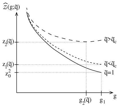
Figure 16: Inverse of the Laplace transformed partition function $\widehat{{\cal Z}}(g;\widetilde{q})$ of the two replica system at various values of the common bond interaction $\widetilde{q}$: The solid line shows the free system without any interaction of common bonds. In the presence of an interaction, the inverse function of the partition function can be obtained by adding a linear function to the free system function. If the interaction is not too strong ($\widetilde{q}<\widetilde{q}_{\mathrm{c}}$, short dashed line) adding the linear function with a small slope does not change the qualitative form of the partition function. In this case, the two replica system is controlled by the singularity at $g={g_{1}}$ which is independent of $\widetilde{q}$. At stronger interactions ($\widetilde{q}>\widetilde{q}_{\mathrm{c}}$, long dashed line) the inverse function develops a minimum. Beyond this minimum it is not invertible any more and the two replica system is then dominated by the singularity arising from this minimum.

If the final slope $z\prime+q^{2}(\widetilde{q}-1)$ of the right hand side of Eq. (77) is positive the situation becomes much different: Upon adding the linear function, $\widehat{{\cal Z}}(g;\widetilde{q})$ develops a minimum at some position $(g_{2}(\widetilde{q}),z_{2}(\widetilde{q}))$. Thus, the inverse function $\widehat{{\cal G}}(z;\widetilde{q})$ has to be calculated from the left (small $g$) branch of $\widehat{{\cal Z}}(g;\widetilde{q})$ and has a square root singularity at $z_{2}(\widetilde{q})$. This square root singularity implies that the characteristic exponent becomes $\theta=3/2$, consistent with the picture that in this phase the two replicas are locked together and fluctuate as one single effective RNA molecule.

The position $g_{2}(\widetilde{q})$ of the minimum is determined by the root of the derivative, i.e., by

$$-q^{2}(\widetilde{q}-1)=\left.\frac{\mathrm{d}}{\mathrm{d}g}\right|_{g=g_{2}(\widetilde{q})}\!\!\!\!\!\!\!\!\widehat{{\cal Z}}(g;1)=\left[\left.\frac{\mathrm{d}}{\mathrm{d}g}\right|_{z=\widehat{{\cal Z}}(g_{2}(\widetilde{q});1)}\!\!\!\!\!\!\!\!\!\!\!\widehat{{\cal G}}(z;1)\right]^{-1}\!\!\!\!\!\!\!\!.$$ (78)

The corresponding value $\widehat{{\cal Z}}(g_{2}(\widetilde{q});\widetilde{q})$ determines the location of the square root singularity $z_{2}(\widetilde{q})$ of $\widehat{{\cal G}}(z;\widetilde{q})$, i.e., the free energy per length of the two replica problem.

$z_{2}(\widetilde{q})$ can be conveniently expressed in terms of the auxiliary quantity $z_{\mathrm{c}}(\widetilde{q})$ defined through $g_{2}(\widetilde{q})=\widehat{{\cal G}}(z_{\mathrm{c}}(\widetilde{q});1)$ as

$$z_{2}(\widetilde{q}) = \widehat{{\cal Z}}(g_{2}(\widetilde{q});\widetilde{q})$$

$$= \widehat{{\cal Z}}(g_{2}(\widetilde{q});1)+q^{2}(\widetilde{q}-1)g_{2}(\widetilde{q})$$

$$= z_{\mathrm{c}}(\widetilde{q})+q^{2}(\widetilde{q}-1)\widehat{{\cal G}}(z_{\mathrm{c}}(\widetilde{q});1).$$

Comparing this expression with Eq. (75) which is valid for small $\widetilde{q}$, we can summarize the complete solution in terms of

$$z_{\mathrm{c}}(\widetilde{q})\!=\!\!\left\{\begin{array}[]{ll}\mbox{the unique $z\in]z_{0}^{2},\infty[$ that ful-}&\widetilde{q}>\widetilde{q}_{\mathrm{c}}\\ \mbox{fils }\frac{\mathrm{d}}{\mathrm{d}z}\widehat{{\cal G}}(z;1)\!=\!\!-\!1\!/[q^{2}(\widetilde{q}\!-\!1)]&\\[10.0pt] z_{0}^{2}=(1+2\sqrt{q})^{2}&\widetilde{q}\leq\widetilde{q}_{\mathrm{c}}\end{array}\right.$$ (79)

where

$$\widetilde{q}_{\mathrm{c}}\equiv 1-\frac{z\prime}{q^{2}}>1,$$ (80)

and

$$z\prime\equiv\frac{1}{\left.\frac{\mathrm{d}}{\mathrm{d}z}\right|_{z=z_{0}^{2}}\widehat{{\cal G}}(z;\widetilde{q}=1)}=-\frac{1}{\sum_{N=1}^{\infty}NG(N)^{2}z_{0}^{-2(N-1)}}.$$ (81)

In terms of this $z_{c}(\widetilde{q})$, the smallest singularity of $\widehat{{\cal Z}}(z;\widetilde{q})$ is located at

$$\zeta(\widetilde{q})=z_{\mathrm{c}}(\widetilde{q})+q^{2}(\widetilde{q}-1)\widehat{{\cal G}}(z_{\mathrm{c}}(\widetilde{q});1).$$ (82)

The free energy per length of the two replica system is given by

$$f=-k_{B}T\ln[z_{\mathrm{c}}(\widetilde{q})+q^{2}(\widetilde{q}-1)\widehat{{\cal G}}(z_{\mathrm{c}}(\widetilde{q});1)]$$ (83)

and the fraction of common bonds is

$$s=\frac{q^{2}\widetilde{q}\widehat{{\cal G}}(z_{\mathrm{c}}(\widetilde{q});1)}{z_{\mathrm{c}}(\widetilde{q})+q^{2}(\widetilde{q}-1)\widehat{{\cal G}}(z_{\mathrm{c}}(\widetilde{q});1)}.$$ (84)

This fraction of common bonds turns out to be continuous at the phase transition but it exhibits a jump in its slope at $\widetilde{q}=\widetilde{q}_{c}$.

In the case $\widetilde{q}\leq\widetilde{q}_{\mathrm{c}}$, these simplify to Eqs. (75) and (76) (or Eqs. (34) and (35) respectively), with $z_{\mathrm{c}}(\widetilde{q})=z_{0}^{2}$ independent of $\widetilde{q}$. The type of singularity of the Laplace transformed partition function is the same as at $\widetilde{q}=1$, resulting in $\theta=3$. For $\widetilde{q}>\widetilde{q}_{\mathrm{c}}$, we cannot write down a closed form expression for $\zeta(\widetilde{q})$ any more. But it is given implicitly in terms of the solution of Eq. (79); it involves only single replica quantities and can thus be evaluated numerically. Moreover, we have seen that the dominant singularity is in this regime a square root singularity implying $\theta=3/2$.

Appendix C The free energy of the two-replica problem

In this appendix we give a derivation of the position of the non-trivial singularity in the Laplace transform of the partition function $\widehat{{\cal G}}(z;\widetilde{q})$. A more intuitive, graphical derivation of this result was given in App. B. Using Eq. (77), we start by calculating

$$\frac{\mathrm{d}}{\mathrm{d}z}\widehat{{\cal G}}(z;\widetilde{q}) = \left[\left.\frac{\mathrm{d}}{\mathrm{d}g}\right|_{g=\widehat{{\cal G}}(z;\widetilde{q})}\!\!\!\!\widehat{{\cal Z}}(g;\widetilde{q})\right]^{-1}$$

$$= \left[\left.\frac{\mathrm{d}}{\mathrm{d}g}\right|_{g=\widehat{{\cal G}}(z;\widetilde{q})}\!\!\!\!\widehat{{\cal Z}}(g;1)+q^{2}(\widetilde{q}-1)\right]^{-1}$$

$$= \left[\left[\left.\frac{\mathrm{d}}{\mathrm{d}z}\right|_{z=\widehat{{\cal Z}}(\widehat{{\cal G}}(z;\widetilde{q});1)}\!\!\!\!\widehat{{\cal G}}(z;1)\right]^{-1}\!\!\!\!\!\!\!\!\!+q^{2}(\widetilde{q}-1)\right]^{-1}\!\!\!\!.$$

This expression obviously has a singularity at $z_{2}(\widetilde{q})$ which is defined by

$$\left.\frac{\mathrm{d}}{\mathrm{d}z}\right|_{z=\widehat{{\cal Z}}(\widehat{{\cal G}}(z_{2}(\widetilde{q});\widetilde{q});1)}\widehat{{\cal G}}(z;1)=-\frac{1}{q^{2}(\widetilde{q}-1)}.$$ (85)

Since $\frac{\mathrm{d}}{\mathrm{d}z}\widehat{{\cal G}}(z;1)\in[1/z\prime,0[$, this is only possible for

$$\widetilde{q}\geq\widetilde{q}_{\mathrm{c}}\equiv 1-\frac{z\prime}{q^{2}}.$$

For smaller values of $\widetilde{q}$, there is no other singularity and the free energy per length is given by Eq. (75).

If $\widetilde{q}\geq\widetilde{q}_{\mathrm{c}}$ the additional singularity $z_{2}(\widetilde{q})$ exists and is — as we will see below — always smaller than the singularity $z_{1}(\widetilde{q})$. Thus, the free energy per length is given by the singularity $z_{2}(\widetilde{q})$ in the strong coupling phase, i.e., for $\widetilde{q}\geq\widetilde{q}_{\mathrm{c}}$.

On the first sight, Eq. (85) still looks as if $z_{2}(\widetilde{q})$ could only be calculated if the full function $\widehat{{\cal G}}(z;\widetilde{q})$ is known. However, for any $\widetilde{q}\geq\widetilde{q}_{\mathrm{c}}$ we can define $z_{\mathrm{c}}(\widetilde{q})$ to be the unique solution of the equation

$$\left.\frac{\mathrm{d}}{\mathrm{d}z}\right|_{z=z_{\mathrm{c}}(\widetilde{q})}\widehat{{\cal G}}(z;1)=-\frac{1}{q^{2}(\widetilde{q}-1)}.$$

This quantity depends only on the function $\widehat{{\cal G}}(z;1)$. According to Eq. (85), $z_{2}(\widetilde{q})$ and $z_{\mathrm{c}}(\widetilde{q})$ are related by $\widehat{{\cal Z}}(\widehat{{\cal G}}(z_{2}(\widetilde{q});\widetilde{q});1)=z_{\mathrm{c}}(\widetilde{q})$. This implies that $\widehat{{\cal G}}(z_{2}(\widetilde{q});\widetilde{q})=\widehat{{\cal G}}(z_{\mathrm{c}}(\widetilde{q});1)$. On the other hand, Eq. (77) applied to $g=\widehat{{\cal G}}(z_{2}(\widetilde{q});\widetilde{q})$ yields

$$z_{2}(\widetilde{q}) = \widehat{{\cal Z}}(\widehat{{\cal G}}(z_{2}(\widetilde{q});\widetilde{q});\widetilde{q})$$

$$= \widehat{{\cal Z}}(\widehat{{\cal G}}(z_{2}(\widetilde{q});\widetilde{q});1)+q^{2}(\widetilde{q}-1)\widehat{{\cal G}}(z_{2}(\widetilde{q});\widetilde{q})$$

$$= z_{\mathrm{c}}(\widetilde{q})+q^{2}(\widetilde{q}-1)\widehat{{\cal G}}(z_{\mathrm{c}}(\widetilde{q});1)$$

which is finally an expression which involves only quantities of the non-interacting system. Since $z+q^{2}(\widetilde{q}-1)\widehat{{\cal G}}(z;1)=\widehat{{\cal Z}}(\widehat{{\cal G}}(z;1);\widetilde{q})$ is a monotonous function on the interval $[z_{0}^{2},z_{\mathrm{c}}(\widetilde{q})]$, we always have $z_{2}(\widetilde{q})\leq z_{1}(\widetilde{q})$ with equality if and only if $z_{\mathrm{c}}(\widetilde{q})=z_{0}^{2}$, i.e., for $\widetilde{q}=\widetilde{q}_{\mathrm{c}}$. Therefore, the free energy per length is indeed given by

$$f_{2}=-k_{B}T\ln[z_{\mathrm{c}}(\widetilde{q})+q^{2}(\widetilde{q}-1)\widehat{{\cal G}}(z_{\mathrm{c}}(\widetilde{q});1)]$$

for any $\widetilde{q}\geq\widetilde{q}_{\mathrm{c}}$.

References

- (1) see, e.g., W. Saenger, Principles of nucleic acid structure (Springer-Verlag, New York, 1984) or B. Alberts et al., Molecular Biology of the Cell (Garland Publishing, New York, 1994).
- (2) see, e.g., R.F. Gesteland and J.F. Atkins eds., The RNA world : the nature of modern RNA suggests a prebiotic RNA world (Cold Spring Harbor Laboratory Press, Cold Spring Harbor, 1993).
- (3) K.A. Dill et al., Protein Sci. 4, 561 (1995).
- (4) J.N. Onuchic, Z. Luthey-Schulten, and P.G. Wolynes, Annu. Rev. Phys. Chem. 48, 545 (1997).
- (5) T. Garel, H. Orland, and E. Pitard, J. Phys. I 7, 1201 (1997).
- (6) E.I. Shakhnovich, Curr. Op. Struct. Biol. 7, 29 (1997).
- (7) for a review see P.G. Higgs, Quart. Rev. Biophys. 33, 199–253 (2000).
- (8) M. Zuker and P. Stiegler, Nucl. Acid. Res. 9, 133–148 (1981).
- (9) J.S. McCaskill, Biopolymers 29, 1105–1119 (1990).
- (10) I.L. Hofacker, W. Fontana, P.F. Stadler, S. Bonhoeffer, M. Tacker, and P. Schuster, Monatshefte f. Chemie 125, 167–188 (1994).
- (11) S.M. Freier, R. Kierzek, J.A. Jaeger, N. Sugimoto, M.H. Caruthers, T. Neilson, and D.H. Turner, Proc. Natl. Acad. Sci. USA 83, 9373–9377 (1986).
- (12) I. Tinoco Jr and C. Bustamante, J. Mol. Biol. 293 271–281 (1999) and references therein.
- (13) B. Maier, D. Bensimon, and V. Croquette, Proc. Natl. Acad. Sci. USA 97, 12002–12007 (2000).
- (14) P.G. de Gennes, Biopolymers 6, 715 (1968).
- (15) P.G. Higgs, Phys. Rev. Lett. 76, 704–707 (1996).
- (16) R. Bundschuh and T. Hwa, Phys. Rev. Lett. 83, 1479–1483 (1999).
- (17) A. Pagnani, G. Parisi, and F. Ricci-Tersenghi, Phys. Rev. Lett. 84, 2026–2029 (2000).
- (18) A.K. Hartmann, Phys. Rev. Lett. 86, 1382–1382 (2001).
- (19) A. Pagnani, G. Parisi, and F. Ricci-Tersenghi, Phys. Rev. Lett. 86, 1383–1383 (2001).
- (20) see, e.g., P. Young ed., Spin glasses and random fields (World Scientific, Singapore, 1998).
- (21) D. Moroz and T. Hwa, in preparation.
- (22) M.S. Waterman, Advan. in Math. Suppl. Studies 1, 167–212 (Academic Press, New York, 1978).
- (23) see, e.g., M. Mitas, Nucl. Acids Res. 25, 2245-2254 (1997).
- (24) see, e.g., W. Feller, An Introduction to Probability Theory and Its Applications (John Wiley & Sons, New York, 1950).
- (25) T.C. Lubensky, J. Isaacson, and S.P. Obukhov, J. Physique 42, 1591–1601 (1981).
- (26) S.F. Edwards and P.W. Anderson, J. Phys. F5, 965 (1975).
- (27) see, e.g., M. Mézard, G. Parisi, and M.A. Virasoro, Spin Glass Theory and Beyond (World Scientific, Singapore, 1986).
- (28) R. Arratia, L. Gordon, and M. Waterman, Ann. Stat. 18, 539–570 (1990).
- (29) D.A. Huse and D.S. Fisher, J. Physique I 1, 621–625 (1991).
- (30) S.R. Morgan and P.G. Higgs, J. Chem. Phys. 105, 7152–7157 (1996).
- (31) S.R. Morgan and P.G. Higgs, J. Phys. A: Math. Gen. 32, 3153–3170 (1998).
- (32) C. Flamm, W. Fontana, I.L. Hofacker, and P. Schuster, RNA 6, 325–338 (2000).
- (33) H. Isambert and E.D. Siggia, Proc. Natl. Acad. Sci. USA 97, 6515–6520 (2000).
- (34) U. Gerland, R. Bundschuh, and T. Hwa, in preparation.
- (35) J.L. Cardy and S. Ostlund, Phys. Rev. B 25, 6899–6909 (1982).
- (36) S.E. Korshunov, Phys. Rev. B 48, 3969–3975 (1993).
- (37) T. Hwa and D. Fisher, Phys. Rev. B 49, 3136–3154 (1994).
- (38) L.-H. Tang and H. Chaté, Phys. Rev. Lett. 86, 830 (2001).
- (39) H. Isambert, personal communication.
- (40) J. Zinn-Justin, Quantum field theory and critical phenomena (Oxford University Press, United Kingdom, 1989).