Scenario of strongly non-equilibrium Bose-Einstein condensation

Abstract

Large scale numerical simulations of the Gross-Pitaevskii equation are used to elucidate the self-evolution of a Bose gas from a strongly non-equilibrium initial state. The stages of the process confirm and refine the theoretical scenario of Bose-Einstein condensation developed by Svistunov, Kagan, and Shlyapnikov svist ; kss ; ks1 : the system evolves from the regime of weak turbulence to superfluid turbulence via states of strong turbulence in the long-wavelength region of energy space.

I Introduction

I.1 Statement of the problem

The experimental realization of Bose-Einstein condensates (BEC) in dilute alkali and hydrogen gases bec1 and more recently in a gas of metastable helium bec2 has stimulated a great interest in the dynamics of BEC. In the case of a pure condensate, both equilibrium and dynamical properties of the system can be described by the Gross-Pitaevskii equation (GPE)gp (in nonlinear physics this equation is known as defocusing nonlinear Schrödinger equation). The GPE has been remarkably successful in predicting the condensate shape in an external potential, the dynamics of the expanding condensate cloud, the motion of quantized vortices; it is also a popular qualitative model of superfluid helium.

An important and often overlooked feature of the GPE is that it gives an accurate microscopic description of the formation of BEC from the strongly degenerate gas of weakly interacting bosons ly ; ks2 . By large scale numerical simulations of the GPE it is possible, in principle, to reveal all the stages of this evolution from weak turbulence to superfluid turbulence with a tangle of quantized vortices as was argued by Svistunov, Kagan, and Shlyapnikov svist ; kss ; ks1 (for a brief review see Ref. svist2, ). This task has up to now remained unfulfilled, though some important steps in this direction have been made in Refs. Damle ; Drummond . We would also like to mention the description of the equilibrium fluctuations of the condensate and highly occupied non-condensate modes using the time-dependent GPE Goral ; Davis .

The goal of this paper is to obtain the conclusive description of the process of strongly non-equilibrium BEC formation in a macroscopically large uniform weakly interacting Bose gas using the GPE. We are especially interested in tracing the development of the so-called coherent regime ly ; svist ; kss ; ks1 at a certain stage of evolution. According to the theoretical predictions kss ; ks1 , this regime sets in after the breakdown of the regime of weak turbulence in a low-energy region of wavenumber space. It corresponds to the formation of the superfluid short-range order which is the state of superfluid turbulence with quasi-condensate local correlation properties.

The notions of weak turbulence and superfluid turbulence are crucial to our understanding of ordering kinetics. In the regime of weak turbulence (for an introduction to the weak turbulence theory for the GPE see Ref. Nazarenko, ), the “single-particle” modes of the field are almost independent due to weak nonlinearity of the system. The smallness of correlations between harmonics in the regime of weak turbulence implies the absence of any order. On the other hand, the regime of superfluid turbulence (for an introduction, see Ref. Donnelly, ) is the regime of strong coherence where the local correlation properties correspond to the superfluid state, but the long-range order is absent because of the presence of a chaotic vortex tangle and non-equilibrium long-wave phonons ks1 . In the case of a weakly interacting, gas the local superfluid order is synonymous to the existence of quasi-condensate correlation properties kss . In a macroscopically large system, the cross-over from weak turbulence to superfluid turbulence is a key ordering process. Indeed, in the regime of weak turbulence there is no order at all, while in the regime of superfluid turbulence the (local) superfluid order has already been formed. Meanwhile, a rigorous theoretical as well as numerical or experimental studies of this stage of evolution have been lacking. The general conclusions concerning this stage kss ; ks1 were made on the basis of qualitative analysis that naturally contained ad hoc elements. The difficulty with an accurate analysis of the transition from weak turbulence to superfluid turbulence comes from the fact that the evolution between these two qualitatively different states takes place in the regime of strong turbulence which is hardly amenable to analytical treatment. Large computational resources are necessary for a numerical analysis of this stage since the problem involves significantly different length scales and, therefore, requires high spatial resolution.

In the present paper we demonstrate that this problem can be unambiguously solved with a powerful enough computer. Our numerics clearly reveal the dramatic process of transformation from weak turbulence to superfluid turbulence and, thus, fills in a serious gap in rigorous theoretic description of the strongly non-equilibrium BEC formation kinetics in a macroscopic system.

The paper is organized as follows. In Sec. I.2 we discuss the relevance of the time-dependent GPE to the description of the BEC formation kinetics and its relation to the other formalisms. In Sec. I.3 we render some important details of the evolution scenario that we are going to observe. In Sec. II we describe our numerical procedure. In Sec. III we present the results of our simulations. In Sec. IV we conclude with outlining the observed evolution scenario and making a comment on the case of a confined gas.

I.2 Time-dependent Gross-Pitaevskii equation and BEC formation kinetics

In this Section we will discuss the question of applicability of the GPE to the BEC formation kinetics, and its connections to the other—full-quantum—treatments. These discussion is especially relevant in the wake of a recent controversy on the applicability of the classical-field description to a non-condensed bosonic field.

A general analysis of the kinetics of a weakly interacting bosonic field was performed in Ref. cd, . In terms of the coherent-state formalism, it was demonstrated that if the occupation numbers are large and somewhat uncertain (with the absolute value of the uncertainty being much larger than unity and with a relative value of the uncertainty being arbitrarily small), then the system evolves as an ensemble of classical fields with corresponding classical-field action. (For an elementary demonstration of this fact for a weakly interacting Bose gas and especially for the discussion of the structure of the initial state see Ref. ks2, .) This has a direct analogy with the electro-magnetic field: (i) the density matrix of a completely disordered weakly interacting Bose gas with large and somewhat uncertain occupation numbers is almost diagonal in the coherent-state representation, so that the initial state can be viewed as a mixture or statistical ensemble of coherent states; (ii) to the leading order each coherent state evolves along its classical trajectory which in our case is given by the GPE

$${\rm i}\hbar{\partial\psi\over\partial t}=-{\frac{\hbar^{2}}{2m}}\nabla^{2}\psi+U|\psi|^{2}\psi,$$ (1)

where $\psi$ is the complex-valued classical field that specifies the index of the coherent state, $m$ is the mass of the boson, $U=4\pi\hbar^{2}a/m$ is the strength of the $\delta$-function interaction (pseudo-)potential, and $a$ is the scattering length. [Note that in a strongly interacting system it is impossible to divide single-particle modes into highly occupied and practically empty ones, so the requirement of weak interactions is essential here. In a strongly interacting system, there are always quantum modes with occupation numbers of order unity that are coupled to the rest of the system.] Therefore, the behavior of the quantum field is equivalent to that of an ensemble of classical matter fields.

It is important to emphasize that in the context of the strongly non-equilibrium BEC formation kinetics the condition of large occupation numbers is self-consistent: the evolution leads to an explosive increase of occupation numbers in the low-energy region of wavenumber space svist where the ordering process takes place. Even if the occupation numbers are of order unity in the initial state, so that the classical matter field description is not yet applicable, the evolution that can be described at this stage by the standard Boltzmann quantum kinetic equation inevitably results in the appearance of large occupation numbers in the low-energy region of the particle distribution (see, e.g., Ref. semikoz ). The blow-up scenario svist indicates that only low-energy part of the field is initially involved in the process. Therefore, one can switch from the kinetic equation to the matter field description for the long-wavelength component of the field at a certain moment in the evolution when the occupation numbers become appropriately large. As the time scale of the formation of the local quasi-condensate correlations is much smaller than any other characteristic time scale of evolution kss , the cut-off of the high-frequency modes, associated with the matter field description, is not important. By the time the interactions (particle exchange) between the high- and low-frequency modes became significant, the local superfluid order had already been developed. The order of interaction wavelengths is of typical thermal deBroglier wavelength and, therefore, these interactions are essentially local with respect to the quasi-condensate and can be described in terms of the kinetic equationsvist ; semikoz .

The thesis of the applicability of the matter field description at large occupation numbers was justified by the analysis of Ref. cd, . Later Stoof questioned the validity of this thesis by introducing the concept of “quantum nucleation” of condensate as a result of an essentially quantum instability Stoof ; the path-integral version of Keldysh formalism was used to substantiate this concept. For a criticism of the concept of “quantum nucleation” see Refs. ks2, ; commentStoof, .

It is important to emphasize, however, that the path-integral approach developed in Stoof appears to be the most fundamental, powerful, and universal way of deriving the basic equations for the dynamics of a weakly interacting Bose gas. In particular, we believe that the demonstration of the applicability of the time-dependent GPE to the description of highly occupied single-particle modes of a non-condensed gas within this formalism would be the most natural since the effective action for the bosonic field is simply the classical-field action of the GPE. Basically, one simply has to make sure that for the modes with large and somewhat uncertain occupation numbers the main contribution to the path integral comes from a close vicinity of the classical trajectories with the quantum corrections being relevant only on large enough times of evolution.

An interesting all-quantum description of the BEC kinetics was implemented in Ref. Drummond, . This technique is based on associating the quantum-field density matrix in coherent-state representation with a correlator of a pair of classical fields which evolution is governed by a system of two coupled nonlinear equations with stochastic terms. Using this method the authors performed a numerical simulation of the BEC formation in a trapped gas of a moderate size. We believe (in particular, in view of general results of Refs. cd, ; ks2, ) that this approach might be further developed analytically to demonstrate explicit overlapping with the other treatments and with the time-dependent GPE. Indeed, the form of the system of two coupled equations of Ref. Drummond, is reminiscent of that of the GPE. This suggests that under the condition of large occupation numbers the system can be decoupled leading to the GPE for the diagonal part of the density matrix with relative smallness of the non-diagonal terms. If the standard Boltzmann equation is applicable, so that the system can be viewed as an ensemble of weakly coupled elementary modes Gardiner , it is natural to expect that the equations of Ref. Drummond, should lead to the kinetic equation. A natural way for deriving kinetic equation from the dynamic equations of Ref. Drummond, is to utilize the standard formalism of the weak turbulence theory. In the case of the GPE, the weak turbulence approximation leads to the quantum-field Boltzmann kinetic equation without spontaneous scattering processes (see, e.g., Ref.Nazarenko ; note also that it is the simplest way to make sure that the GPE is immediately applicable once the occupation numbers are large). It is natural to expect that in the full-quantum treatment of Ref. Drummond, the weak-turbulence procedure over the dynamic equations would result in the complete quantum-field Boltzmann kinetic equation with the spontaneous processes retained. Unfortunately, we are not aware of such investigations of the equations of Ref. Drummond, that might be very instructive for the general understanding of the dynamics of a weakly interacting Bose gas.

I.3 Initial state and evolution scenario

In what follows we consider the evolution of Eq. (1) starting with a strongly non-equilibrium initial condition

$$\psi({\bf r},t=0)=\sum_{\bf k}a_{\bf k}\exp({\rm i}{\bf kr}),$$ (2)

where the phases of the complex amplitudes $a_{\bf k}$ are distributed randomly. Such an initial condition follows from the microscopic quantum-mechanical analysis of the state of a weakly interacting Bose gas in the kinetic regime ks2 . Theoretical investigations of the relaxation of such an initial state towards the equilibrium configuration were performed by Svistunov, Kagan, and Shlyapnikov svist ; kss ; ks1 . The analysis revealed a number of stages in the evolution. Initially the system is in the weak turbulence regime and thus can be described by Boltzmann kinetic equation. The kinetic equation is obtained as the random-phase approximation of Eq. (1) for occupation numbers $n_{\bf k}$ defined by $\langle a_{\bf k}a_{\bf k^{\prime}}^{*}\rangle\approx n_{\bf k}\delta_{\bf k}\delta_{\bf k^{\prime}}$. Alternatively, the weak-turbulence kinetic equation follows from the general quantum Boltzmann kinetic equation if one neglects spontaneous scattering as compared with stimulated scattering (because of large occupation numbers). Svistunov svist and later Semikoz and Tkachev semikoz considered the self-similar solution of the Boltzmann kinetic equation:

$$n_{\epsilon}(t) = A\epsilon_{0}^{-\alpha}(t)f(\epsilon/\epsilon_{0}),\qquad t\leq t_{*},$$ (3)

$$\epsilon_{0}(t) = B(t_{*}-t)^{1/2(\alpha-1)},$$ (4)

$$f(x) \rightarrow x^{-\alpha}\quad{\rm at}\quad x\rightarrow\infty,\quad f(0)=1,$$ (5)

where $\epsilon=\hbar^{2}k^{2}/2m$. The dimensional constants $A$ and $B$ relate to each other by $(\alpha-1)m^{3}U^{2}A^{2}=\lambda\pi^{3}\hbar^{7}B^{2(\alpha-1)}$, where the parameters $\alpha$ and $\lambda$ were determined by numerical analysis as $\alpha\approx 1.24$ semikoz and $\lambda\approx 1.2$ svist . The form of the function $f$ was also determined numerically in Ref. svist . The solution (3)-(5) has only one free parameter, say $A$, that depends on conditions in the “pre-historic” evolution. By “pre-historic” evolution we mean any sort of non-universal dynamics preceding the appearance of self-similarity. This dynamics is sensitive to the details of the initial condition or/and cooling mechanism as well as to the spontaneous-scattering terms in the kinetic equation which cannot be neglected until the occupation numbers are large enough. When the self-similar regime sets in at a certain step of evolution all the particular details of the previous evolution are absorbed in the single parameter $A$.

The self-similar solution (3)-(5) describes a wave in energy space propagating from high to lower energies. The energy $\epsilon_{0}(t)$ defines the “head” of the wave. The wave propagates in a blow-up fashion: $\epsilon_{0}(t)\rightarrow 0$ and $n_{\epsilon_{0}}(t)\rightarrow\infty$ as $t\rightarrow t_{*}$. In reality the validity of the kinetic equations associated with the random phase approximation breaks down shortly before the blow-up time $t_{*}$. This moment marks the beginning of a qualitatively different stage in the evolution the coherent regime: strong turbulence evolves into a quasi-condensate state. In the coherent regime the phases of the complex amplitudes $a_{\bf k}$ of the field $\psi$ become strongly correlated and the periods of their oscillations are then comparable with the evolution times of the occupation numbers. The formation of the quasi-condensate is manifested by the appearance of a well-defined tangle of quantized vortices and, therefore, by the beginning of the final stage of the evolution: superfluid turbulence. In this regime the vortex tangle starts to relax over macroscopically large times.

II Numeric procedure

II.1 Finite-difference scheme

We performed a large scale numerical integration of a dimensionless form of the GPE

$$-2{\rm i}{\partial\psi\over\partial t}=\nabla^{2}\psi+|\psi|^{2}\psi,$$ (6)

starting with a strongly non-equilibrium initial condition. Our calculations were done in a periodic box $N^{3}$, with $N=256$, using a fourth-order (with respect to the spatial variables) finite-difference scheme. The scheme corresponds to the Hamiltonian system in the discrete variables $\psi_{ijk}$:

$${\rm i}{\partial\psi_{ijk}\over\partial t}={\partial H\over\partial\psi^{*}_{ijk}}\;,$$ (7)

where

$$H={\frac{1}{2}}\sum_{ijk} \psi^{*}_{ijk} [-\textstyle{{\frac{1}{12}}}(\psi_{i+2,j,k}-\psi_{i-2,j,k}$$

$$+ \psi_{i,j+2,k} -\psi_{i,j-2,k}+\psi_{i,j,k+2}-\psi_{i,j,k-2})$$

$$+\textstyle{{\frac{4}{3}}}( \psi_{i+1,j,k} -\psi_{i-1,j,k}+\psi_{i,j+1,k}-\psi_{i,j-1,k}$$

$$+ \psi_{i,j,k+1} -\psi_{i,j,k-1})]-\textstyle{{\frac{1}{2}}}|\psi_{ijk}|^{4}$$ (8)

[in the numerics we set the space step in each direction of the grid as $dx=dy=dz=1$].

Equation (7) conserves the energy $H$ and the total particle number $\sum_{ijk}|\psi_{ijk}|^{2}$ exactly. In time stepping, the leap-frog scheme was implemented

$${\rm i}{\frac{\psi_{ijk}^{n+1}-\psi_{ijk}^{n-1}}{2dt}}=\Big{(}{\partial H\over\partial\psi^{*}_{ijk}}\Big{)}^{n}\;,$$ (9)

with $dt=0.03$. To prevent the even-odd instability of the leap-frog iterations, we introduce the backward Euler step

$${\rm i}{\frac{\psi_{ijk}^{n+1}-\psi_{ijk}^{n}}{dt}}=\Big{(}{\partial H\over\partial\psi^{*}_{ijk}}\Big{)}^{n+1}\;,$$ (10)

every $10^{4}$ time steps. The leap-frog scheme is nondissipative, so the only loss of energy and of the total particle number occurs during the backward Euler step and, since we take this step very rarely, these losses are insignificant.

The code was tested against known solutions of the GPE: vortex rings and rarefaction pulses jr . The simulations were performed on a Sun Enterprise 450 Server and took about three months to complete for the main set of calculations discussed below.

II.2 Initial condition

To eliminate the computationally expensive (and the least physically interesting) transient regime, we started directly from the self-similar solution Eq. (2) with (3)-(5), so that:

$$a_{\bf k}=\sqrt{\xi_{\bf k}n_{0}f(\epsilon/\epsilon_{0})}\exp[{\rm i}\phi_{\bf k}],$$ (11)

where $\xi_{\bf k}$ and $\phi_{\bf k}$ are random numbers. [Note that in the simulations the momentum ${\bf k}$ is the momentum of the lattice Fourier transform.] The phase $\phi_{\bf k}$ is uniformly distributed on $[0,2\pi]$ in accordance with the basic statement of the theory of weak turbulence and with the explicit microscopic analysis of corresponding quantum field states ks2 . The choice of $\xi_{\bf k}$ is rather arbitrary, we only fix its mean value to be equal to unity, introducing therefore the parameter $n_{0}$. The weak-turbulence evolution is invariant to the details of the statistics of $|a_{\bf k}|$. By the time the system enters the regime of strong turbulence, the proper statistics is established automatically since each harmonic participates in a large number of scattering events. We tried different distributions for $\xi_{\bf k}$ and saw no systematic difference in the evolution picture. The main set of our simulations was done with the distribution function $w(\xi_{\bf k})=\exp{(-\xi_{\bf k})}$ (heuristically suggested by equilibrium Hibbs statistics of harmonics in the non-interacting model).

When choosing the parameters of the initial condition (2) specified by the complex Fourier amplitudes (11), we have to take $\epsilon_{0}$ small enough to be free from systematic error of large finite-differences. On the other hand, taking $\epsilon_{0}$ too small reduces the physical size of the system. Let us define one period of the amplitude oscillation as $t_{p}=2\pi/\epsilon_{0}$ and the number of periods before the blow-up as $P=t_{*}/t_{p}$. When choosing the value of $n_{0}$ in combination with $\epsilon_{0}$, we would like to avoid having $P$ too small when the time scale of the kinetic regime becomes too short, or having $P$ too large, when the finite-size effects (the discreteness of the $\bf k$) dominate the calculation. Given the maximal available grid size $N=256$, we found that it is optimal to take $n_{0}=15$ and $\epsilon_{0}=1/18$, so that $t_{p}\approx 113$, $t_{*}=4\lambda\pi^{3}/(\alpha-1)\epsilon_{0}^{2}n_{0}^{2}\approx 893$, and $P\approx 8$.

III Data processing and results

The instantaneous values of the occupation numbers $n_{\bf k}(t)=|a_{\bf k}(t)|^{2}$ are extremely ‘noisy’ functions of time. To be able to draw some quantitative comparisons and conclusions we need either to perform some averaging or to deal with some coarse-grained self-averaging characteristics of the particle distribution. Taking the second option, we introduce shells in momentum space. By the $i$-th shell ($i=1,2,3,\ldots$) we understand the set of momenta satisfying the condition $i-1\leq\log_{2}(k/2\pi)<i$. The idea behind this definition is that each shell represents some typical momentum (wavelength) scale and thus allows to introduce a coarse-grained characteristic of the occupation numbers corresponding to a given scale. Namely, for each shell $i$ we introduce the mean occupation number $\eta_{i}(t)=\sum^{({\rm shell}~{}i)}n_{\bf k}(t)/M_{i}$, where $M_{i}$ is the number of harmonics in the $i$-th shell. The harmonic ${\bf k}=0$, which plays a special role (at the very end of the evolution), is not assigned to any shell.

Another instructive coarse-grained characteristic of the particle distribution is the integral distribution function $F_{k}=\sum_{k^{\prime}\leq k}n_{{\bf k}^{\prime}}$ which shows how many particles have momenta not exceeding $k$. We use function $F_{k}$ to keep track of the formation of the quasi-condensate and to determine wavenumber span of the above-the-condensate particles. This information is used, in particular, for filtering out the high-frequency harmonics in order to interpret the results of our numerical calculations in superfluid turbulence regime.

With the above-introduced quantities we now turn to the analysis of the results of our numerical simulations. The self-similar character of the evolution is clearly observed in Fig. 1. Inserts in Fig. 1 give the comparison of the theoretical prediction of the evolution of the occupation number function $n_{\epsilon}(t)$ defined by Eq. (3) and the evolution of the first and the second shells. The agreement with the theoretical predictions svist is quite good for $t<600$. After that the numerical solution deviates from the self-similar theoretical solution which is the manifestation of the onset of the strong turbulence stage of evolution.

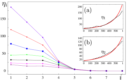
Figure 1: The time evolution of $\eta_{i}(t=100j)$ in the weak turbulence regime for $j=0,\ldots,6$. In the insets we show the theoretical self-similar solution (3)-(5) (solid line) and the solution obtained through the numerical integration of (6) (dashed line) for the shells $i=1$ (a) and $i=2$ (b).

As follows from the dimensional analysis (see, e.g., Ref. svist2 ), the characteristic time, $t_{0}$, and the characteristic wave vector, $k_{0}$, at the beginning of the strong turbulence regime are given by the relations

$$t_{*}-t_{0}\sim C_{0}[\hbar^{2\alpha+5}/m^{3}U^{2}A^{2}]^{1/(2\alpha-1)}\;,$$ (12)

$$k_{0}\sim C_{1}[AU(m/\hbar)^{\alpha+1}]^{1/(2\alpha-1)}\;,$$ (13)

where $C_{0}$ are $C_{1}$ some dimensionless constants. Our numerical results (Fig. 1) indicate that $t_{*}-t_{0}\sim 300$ which implies $C_{0}\sim 40$. After the formation of the quasi-condensate ($t>1000$), the distribution of particles acquires a bimodal shape which is seen in Fig. 2. The salient characteristic of the distribution is the shoulder which becomes sharper and sharper as the evolution continues. Note that by definition of the function $F_{k}$, the height of the shoulder is equal to the number of the quasi-condensate particles. From Fig. 2 we estimate $k_{0}\sim 15$ which means that

$$C_{1}\sim C_{0}\sim 40\;.$$ (14)

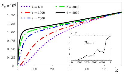
Figure 2: Evolution of the integral distribution of particles $F_{k}=\sum_{k^{\prime}\leq k}n_{{\bf k}^{\prime}}$. Notice the appearance of a ‘shoulder’ of $F_{k}$ indicative of the quasi-condensate formation. The evolution of $n_{{\bf k}=0}$ is presented in the inset. Note the strong fluctuations typical for the evolution of a single harmonic. The fluctuations are also seen in the graph of the first shell (see insert (a) of Fig. 1).

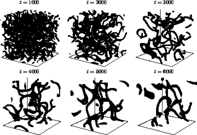
Figure 3: Evolution of topological defects in the phase of the long-wavelength part $\tilde{\psi}$ of the field $\psi$ in the computational box $256^{3}$. The defects are visualized by isosurfaces $|\tilde{\psi}|^{2}=0.05\langle|\tilde{\psi}|^{2}\rangle$. High-frequency spatial waves are suppressed by the factor $\max\{1-k^{2}/k_{c}^{2},0\}$, where the cut-off wave number is chosen according to the phenomenological formula $k_{c}=9-t/1000$.

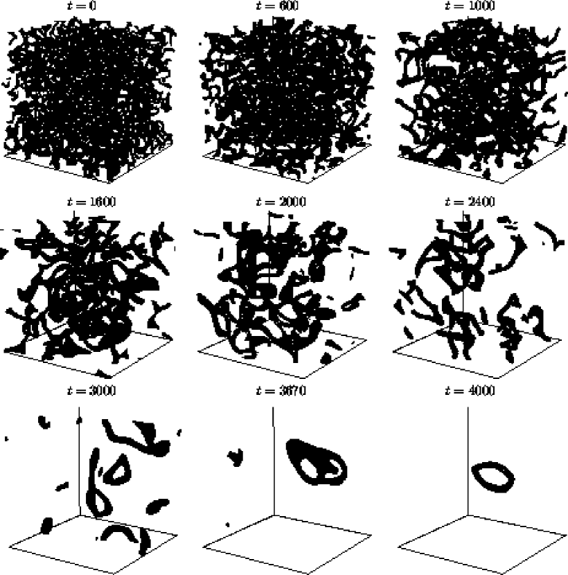
Figure 4: Evolution of topological defects in the phase of the long-wavelength part $\tilde{\psi}$ of the field $\psi$ in the computational box $128^{3}$. The defects are visualized by isosurfaces $|\tilde{\psi}|^{2}=0.05\langle|\tilde{\psi}|^{2}\rangle$. High-frequency spatial waves are suppressed by the factor $\max\{1-k^{2}/k_{c}^{2},0\}$, where the cut-off wave number is chosen according to the phenomenological formula $k_{c}=9-t/1000$.

Within the coherent regime the momentum distribution of the harmonics yields rather incomplete picture of the evolution and it becomes reasonable to follow the ordering process in coordinate space. The tracing the topological defects in the phase of the long-wavelength part of the complex matter field $\psi$ is very important since the transformation of these defects into a tangle of well-separated vortex lines is the most essential feature of the superfluid short-range ordering ks1 . To this end we first filter out the high-frequency harmonics by performing the transformation $a_{\bf k}\rightarrow a_{\bf k}\max\{1-k^{2}/k_{c}^{2},0\}$, where $k_{c}$ is a cut-off wave number. When the function $F_{k}$ has a pronounced quasi-condensate shoulder, the natural choice is to take $k_{c}$ somewhat larger than the momentum of the shoulder in order to remove the above-the-condensate part of the field $\psi$. In the regime of weak turbulence, when there is no quasi-condensate, the procedure of filtering is ambiguous: the distribution is not bimodal, so there is no special low momentum $k_{c}$; also, the structure of the defects in the filtered field essentially depends on the cut-off parameter and, thus, has no physical meaning.

The results of visualizing the topological defects are presented in Fig. 3. The formation of a tangle of well-separated vortices and the decay of superfluid turbulence are clearly seen. This is the key point of our simulation. To the best of our knowledge, this is the first unambiguous demonstration of the formation of the state of superfluid turbulence in the course of self-evolution of weakly interacting Bose gas. This result forms a solid basis for the analysis of the further stages of long-range ordering in terms of well-developed theory of superfluid turbulence that was performed in Ref. ks1, (see also Ref. ks3, ).

The characteristic time of the evolution of the vortex tangle depends on the typical interline spacing, $R$, as $R^{2}/\ln(R/a_{0})$, where $a_{0}$ is the vortex core size (see, e.g., ks1 ). During the final stage of evolution, when $R$ is of the order of linear size of the computational box, the slowing down of the relaxation process makes numerical simulation of the final stage of the vortex tangle decay to be enormously expensive in a large computational box. For example, according to the above-mentioned estimate of the relaxation time, to achieve the complete disappearance of the vortex tangle in our $N=256$ system we would need several years. To observe this final stage of the vortex tangle decay, we repeated the calculations for a smaller computational box with $N=128$ (reducing in this way the computational time by a factor of $\sim 32=2^{3}\times 2^{2}$); see Fig. 4. Parameters of the initial condition are $\epsilon=1/2$ and $n_{0}=2\pi$, so that the number of periods before the blow-up is $P\approx 5$. A single vortex ring remains at $t=4000$ as the result of the turbulence decay; see Fig. 5(a).

Figure 5: Comparison of two isosurfaces obtained by different filtering techniques. The solution at $t=4000$ is obtained by numerical integration of (6) in the periodic box with $N=128$. The isosurface $|\tilde{\psi}|^{2}=0.05\langle|\tilde{\psi}|^{2}\rangle$ is plotted in Fig. 5(a) using the high-frequency filtering with $k_{c}=5$. The isosurface $|\widehat{\psi}|^{2}=0.2\langle|\widehat{\psi}|^{2}\rangle$ is plotted in Fig. 5(b), where $\widehat{\psi}$ is defined by Eq.(15).

The above-mentioned filtering method allows us to visualize the position of the core of a quantized vortex line, but not the actual size of the core since we force the solution to be represented by a relatively small number of harmonics. To get a better representation of an actual size of the core as well as to resolve another objects of interest—rarefaction pulses jr , which are likely to appear in the course of transformation of strong turbulence into superfluid turbulence, we implement a different type of filtering based on time averaging. We introduce a Gaussian-weighted time average of the field $\psi$:

$$\widehat{\psi}_{ijk}(t)=\int\psi_{ijk}(\tau)\exp[-(\tau-t)^{2}/100]\,d\tau\;.$$ (15)

The width of the Gaussian kernel in (15) is chosen in such a way that the (disordered) high-frequency part of the field $\psi$ is averaged out revealing the strongly correlated low-frequency part $\widehat{\psi}$. Fig. 5 compares the density isosurfaces obtained by two different methods: by high-frequency suppression (Fig. 5a) and by time averaging (Fig. 5b). In the latter case we reveal the actual shape of the vortex core and resolve the rarefaction pulses.

IV Conclusion

We have performed large scale numerical simulations of the process of strongly non-equilibrium Bose-Einstein condensation in a uniform weakly interacting Bose gas. In the limit of weak interaction under the condition of strong enough deviation from equilibrium the key stage of ordering dynamics—superfluid turbulence formation—is universal and corresponds to the process of self-ordering of a classical matter field which dynamics is governed by the time-dependent Gross-Pitaevskii equation (defocusing nonlinear Schrödinger equation). The universality implies independence of evolution from the details of initial processes such as, for example, cooling mechanism and rate as well as from quantum effects such as spontaneous scattering. All the information about the evolution preceding the universal stage is absorbed in the single parameter $A$ that defines scaling of characteristic time and wavenumber, in accordance with Eqs. (12)-(14).

The most important features of the BEC formation scenario observed in our simulation are as follows. The low-energy part of the quantum field characterized by large occupation numbers and, thus, described by a classical complex matter field $\psi$ obeying Eq. (1) initially evolves in a weak-turbulent self-similar fashion according to Eqs. (3)-(5). The occupation numbers at small energies become progressively larger. At the characteristic time moment $t_{0}$, given by Eq. (12), close to the formal blow-up time $t_{*}$ of the solution (3)-(5), the self-similarity of the energy distribution breaks down. The distribution gradually becomes bimodal; the low-energy quasi-condensate part of the field sets to the state of superfluid turbulence characterized by a tangle of the vortex lines. The further evolution of the quasi-condensate is independent of the rest of the system (apart from a permanent flux of the particles into the quasi-condensate) and basically is the process of relaxation of superfluid turbulence. All vortex lines relax in a macroscopically large time.

In the present paper, we dealt with the case of macroscopically large uniform system. As far as the case of a trapped gas is concerned, the situation becomes sensitive to the competition between finite size and nonlinear effects. If nonlinear effects dominate, the basic physics of the ordering process is predicted to be analogous to that revealed by our simulation svist3 . If finite-size effects dominate (which means that the initial size of the condensate is smaller than corresponding healing length, so that, for example, vortices cannot arise in principle svist3 ), the ordering kinetics is substantially simplified being reduced to the growth of genuine condensate Gardiner ; Bijlsma . Clearly, our numerical approach can be extended to the case of a trapped Bose gas by simply including a term with an external potential in Eq. (1). Such a simulation could provide a deeper interpretation of the first experiments on the kinetics of BEC formation Miesner ; Kohl answering, in particular, the question of whether the process involves the formation of vortex tangle; and if not, under which conditions one may expect formation of superfluid turbulence (quasi condensate) in a realistic experimental situation.

- (1) B.V. Svistunov, J. Moscow Phys. Soc. 1, 373 (1991).
- (2) Yu. Kagan, B.V. Svistunov, and G.V. Shlyapnikov, Zh. Eksp. Teor. Fiz. 101, 528 (1992) [Sov. Phys. JETP 75, 387 (1992)].
- (3) Yu. Kagan and B.V. Svistunov, Zh. Eksp. Theor. Fiz. 105, 353 (1994) [Sov. Phys. JETP 78, 187 (1994)].
- (4) M.H. Anderson et al., Science 269, 198 (1995); K.B. Davis et al., Phys. Rev. Lett. 75, 3969 (1995); C.C. Bradley et al., Phys. Rev. Lett. 78, 985 (1997).
- (5) A. Robert et al., Science Express 10.1126/science. 1060622 (2001); F. Pereira Dos Santos et al., Phys. Rev. Lett. 86, 3459 (2001).
- (6) V.L. Ginzburg and L.P. Pitaevskii, Zh. Eksp.Teor. Fiz. 34, 1240 (1958) [Sov. Phys. JETP 7, 858 (1958)]; E.P. Gross, Nuovo Cimento 20, 454 (1961); L.P. Pitaevskii, Soviet Physics JETP, 13, 451 (1961).
- (7) E. Levich and V. Yakhot, J. Phys. A: Math. Gen. 11, 2237 (1978).
- (8) Yu. Kagan and B.V. Svistunov, Phys. Rev. Lett. 79, 3331 (1997).
- (9) B.V. Svistunov, Kinetics of Strongly Non-Equilibrium Bose-Einstein Condensation, in Quantized Vortex Dynamics and Superfluid Turbulence (Lecture Notes in Physics, Vol. 571), Eds. C.F. Barenghi, R.J. Donnelly, and W.F. Vinen, Springer-Verlag, 2001 (cond-mat/0009368).
- (10) K. Damle, S.N. Majumdar, and S. Sachdev, Phys. Rev. A 54, 5037 (1996).
- (11) P.D. Drummond and J.F. Corney, Phys. Rev. A, 60, R2661 (1999). The all-quantum simulation performed in this paper is similar to solving the GPE.
- (12) K. Góral, M. Gajda, and K. Rza̧żewski, Opt. Exp. 8, 92 (2001).
- (13) M.J. Davis, S.A. Morgan, and K. Burnett, Phys. Rev. Lett. 87, 160402 (2001).
- (14) S. Nazarenko, Yu. Lvov, and R. West, Weak Turbulence Theory for the Gross-Pitaevskii Equation in Quantized Vortex Dynamics and Superfluid Turbulence (Lecture Notes in Physics, Vol. 571), Eds. C.F. Barenghi, R.J. Donnelly, and W.F. Vinen, Springer-Verlag, 2001.
- (15) R.J. Donnelly, Quantized Vortices in He II (Cambridge Studies in Low Temperature Physics Vol. 3), Cambridge University Press, 1991; C.F. Barenghi, R.J. Donnelly, and W.F. Vinen (Eds.), Quantized Vortex Dynamics and Superfluid Turbulence (Lecture Notes in Physics, Vol. 571), Springer-Verlag, 2001.
- (16) P. Carruthers and K.S. Dy, Phys. Rev. 147, 214 (1966).
- (17) D.V. Semikoz and I.I. Tkachev, Phys. Rev. D 55, 489 (1997).
- (18) H.T.C. Stoof, J. Low Temp. Phys. 114, 11 (1999); and earlier papers by the same author cited therein.
- (19) In Stoof it was argued that the quantum instability leads to a spontaneous formation of a homogeneous condensate on extremely short time scale. The evidence of this instability was presented using the path-integral version of Keldysh formalism developed for the Bose gas. The appearance of a term that corresponds to a uniform time-dependent external field in the effective action and changes its sign was used as the indicator of this instability. Notice, however, that in the non-Euclidean case under consideration such a term can be immediately absorbed into the phase of the field and, therefore, cannot effect the evolution.
- (20) C.W. Gardiner et al. Phys. Rev. Lett. 81, 5266 (1998); M.J. Davis, C.W. Gardiner, and R.J. Ballagh, Phys. Rev. A 62, 63608 (2000).
- (21) C.A. Jones and P.H. Roberts, J. Phys. A: Gen. Phys. 15, 2599 (1982).
- (22) Yu. Kagan and B.V. Svistunov, Pis’ma Zh. Eksp. Theor. Fiz. 67, 495 (1998) [JETP Lett. 67, 521 (1998)].
- (23) B.V. Svistunov, Phys. Lett. A 287, 169 (2001).
- (24) M.J. Bijlsma, E. Zaremba, and H.T.C. Stoof, Phys. Rev. A 62, 63609 (2000).
- (25) H.-J. Miesner et al., Science 279, 1005 (1998).
- (26) M. Köhl, T.W. Hänsch, and T. Esslinger, cond-mat/0106642.