Introducing Variety in Risk Management

“Yesterday the S&P500 went up by 3%”. Is this number telling all the story if half the stocks went up 5% and half went down 1%? Surely one can do a little better and give two figures, the average and the dispersion around this average, that two of us have recently christened the variety [1].

Call $r_{i}(t)$ the return of asset $i$ on day $t$. The variety ${\cal V}(t)$ is simply the root mean square of the stock returns on a given day:

$${\cal V}^{2}(t)=\frac{1}{N}\sum_{i=1}^{N}\left(r_{i}(t)-r_{m}(t)\right)^{2},$$ (1)

where $N$ is the number of stocks and $r_{m}=(1/N)\sum_{i}r_{i}$ is the market average. If the variety is, say, 0.1%, then most stocks have indeed made between 2.9% and 3.1%. But if the variety is 10%, then stocks followed rather different trends during the day and their average happened to be positive, but this is just an average information.

The variety is not the volatility of the index. The volatility refers to the amplitude of the fluctuations of the index from one day to the next, not the dispersion of the result between different stocks. Consider a day where the market has gone down 5% with a variety of 0.1% – that is, all stocks have gone down by nearly 5%. This is a very volatile day, but with a low variety. Note that low variety means that it is hard to diversify: all stocks behave the same way.

The intuition is however that there should be a correlation between volatility and variety, probably a positive one: when the market makes big swings, stocks are expected to be all over the place. This is actually true. Indeed the correlation coefficient between ${\cal V}(t)$ and $|r_{m}|$ is 0.68. The variety is, on average, larger when the amplitude of the market return is larger (see the discussion below). Very much like the volatility, the variety is correlated in time: there are long periods where the market volatility is high and where the market variety is high (see Fig. 1). Technically, the temporal correlation function of these two objects reveal a similar slow (power-law like) decay with time.

Figure 1 about here

A theoretical relation between variety and market average return can be obtained within the framework of the one-factor model, that suggests that the variety increases when the market volatility increases. The one-factor model assumes that $r_{i}(t)$ can be written as:

$$r_{i}(t)=\alpha_{i}+\beta_{i}{\cal R}_{m}(t)+\epsilon_{i}(t),$$ (2)

where $\alpha_{i}$ is the expected value of the component of security $i$’s return that is independent of the market’s performance (this parameter usually plays a minor role and we shall neglect it), $\beta_{i}$ is a coefficient usually close to unity that we will assume to be time independent, ${\cal R}_{m}(t)$ is the market factor and $\epsilon_{i}(t)$ is called the idiosyncratic return, by construction uncorrelated both with the market and with other idiosyncratic factors. Note that in the standard one-factor model the distributions of ${\cal R}_{m}$ and $\epsilon_{i}$ are chosen to be Gaussian with constant variances, we do not make this assumption and let these distributions be completely general including possible volatility fluctuations.

In the study of the properties of the one-factor model it is useful to consider the variety $v(t)$ of idiosyncratic part, defined as

$$v^{2}(t)={\frac{1}{N}\sum_{i=1}^{N}[\epsilon_{i}(t)]^{2}}.$$ (3)

Under the above assumptions the relation between the variety and the market average return is well approximated by (see Box 1 for details):

$${\cal V}^{2}(t)\simeq v^{2}(t)+\Delta\beta^{2}r_{m}^{2}(t),$$ (4)

where $\Delta\beta^{2}$ is the variance of the $\beta$’s divided by the square of their mean.

Therefore, even if the idiosyncratic variety $v$ is constant, Eq. (4) predicts an increase of the volatility with $r_{m}^{2}$, which is a proxy of the market volatility. Because $\Delta\beta^{2}$ is small, however, this increase is rather small. As we shall now discuss, the effect is enhanced by the fact that $v$ itself increases with the market volatility.

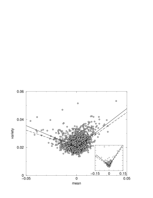
Figure 2: Daily variety $v$ of idiosyncratic terms of the one-factor model (Eq. (3)) as a function of the market average $r_{m}$ of the 1071 NYSE stocks continuously traded from January 1987 to December 1998. Each circle refers to one trading day of the investigated period. In the main panel we show the trading days with $r_{m}$ belonging to the interval from $-0.05$ to $0.05$, whereas in the inset we show the whole data set including five most extreme days. The two solid lines are linear fits over all days of positive (right line) and negative (left line) market average. The slope of the two lines are $+0.55\pm 0.02$ (right) and $-0.30\pm 0.02$ (left). The tick distance in the ordinate of the inset is equal to the one of the main panel. The two dashed lines are linear fits obtained with a robust local M-estimates minimizing the absolute deviation. The slope of the two lines are $+0.51$ (right) and $-0.25$ (left). These values are quite close to the previously obtained ones, showing that the role of outliers is minor.

In its simplest version, the one-factor model assumes that the idiosyncratic part $\epsilon_{i}$ is independent of the market return. In this case, the variety of idiosyncratic terms $v(t)$ is constant in time and independent from $r_{m}$. In Fig. 2 we show the variety of idiosyncratic terms as a function of the market return. In contrast with these predictions, the empirical results show that a significant correlation between $v(t)$ and $r_{m}(t)$ indeed exists. The degree of correlation is different for positive and negative values of the market average. In fact, the best linear least-squares fit between $v(t)$ and $r_{m}(t)$ provides different slopes when the fit is performed for positive (slope $+0.55$) or negative (slope $-0.30$) value of the market average. We have again checked that these slopes are not governed by outliers by repeating the fitting procedure in a robust way. The best fits obtained with this procedure are shown in Fig. 2 as dashed lines. The slopes of the two lines are -0.25 and 0.51 for negative and positive value of the market average, respectively. Therefore, from Eq.(4) we find that the increase of variety in highly volatile periods is stronger than what is expected from the simplest one-factor model, although not as strong for negative (crashes) than it is for positive (rally) days. By analyzing the three largest crashes occurred at the NYSE in the period from January 1987 to December 1998, we observe two characteristics of the variety which are recurrent during the investigated crashes: (i) the variety increases substantially starting from the crash day and remains at a level higher than typical for a period of time of the order of sixty trading days; (ii) the highest value of the variety is observed the trading day immediately after the crash.

Figure 2 about here

An important quantity for risk management purposes is the degree of correlation between stocks. If this correlation is too high, diversification of risk becomes very difficult to achieve. A natural way [2] to characterize the average correlation between all stocks $i,j$ on a given day ${\cal C}(t)$ is to define the following quantity:

$${\cal C}(t)=\frac{\frac{1}{N(N-1)}\sum_{i\neq j}r_{i}(t)r_{j}(t)}{\frac{1}{N}\sum_{i}r_{i}^{2}(t)}.$$ (5)

As shown in the technical Box 1, to a good approximation one finds:

$${\cal C}(t)\simeq\frac{1}{1+F(t)},\qquad F(t)\equiv\frac{v^{2}(t)}{r_{m}^{2}(t)},$$ (6)

As mentioned above, the variety of the idiosyncratic terms is constant in time in the simplest one-factor model. The correlation structure in this version of the one-factor model is very simple and time independent. Still, the quantity ${\cal C}$, taken for a proxy of the correlations on a given day, increases with the ‘volatility’ $r_{m}^{2}$, simply because $F$ decreases. As shown in Fig. 3, the simplest one factor model in fact overestimates this increase [2]. Because the idiosyncratic variety $v^{2}(t)$ tends to increase when $|r_{m}|$ increases (see Figure 2), the quantity $F(t)$ is in fact larger and ${\cal C}$ is smaller. This may suggest that, at odds with the common lore, correlations actually are less effective than expected using a one-factor model in high volatility periods: the unexpected increase of variety gives an additional opportunity for diversification. Other, more subtle indicators of correlations, like the exceedance correlation function defined in Box 2 and shown in Fig. 4 (see [4]), actually confirm that the commonly reported increase of correlations during highly volatile bear periods might only reflect the inadequacy of the indicators that are used to measure them.

Figures 3 and 4 about here

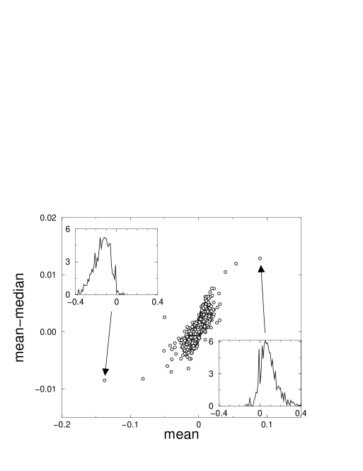
Figure 5: Daily asymmetry ${\cal A}$ of the probability density function of daily returns of a set of 1071 NYSE stocks continuously traded from January 1987 to December 1998 as a function of the market average $r_{m}$. Each circle refers to one trading day of the investigated period. In the insets we show the probability density function of daily returns observed for the two most extreme market days of the period investigated. Specifically, the left inset refers to Black Monday (October 19th, 1987) and the right inset refers to October 21st, 1987. The negative (left inset) and positive (right inset) skewness of the distribution is clearly seen in both cases.

Therefore, the idiosyncrasies are by construction uncorrelated, but not independent of the market. This shows up in the variety, does it also appear in different quantities? We have proposed above to add to the market return the variety as a second indicator. One can probably handle a third one, which gives a refined information of what happened in the market on a particular day. The natural question is indeed: what fraction $f$ of stocks did actually better than the market? A balanced market would have $f=50\%$. If $f$ is larger than $50\%$, then the majority of the stocks beat the market, but a few ones lagging behind rather badly, and vice versa. A closely related measure is the asymmetry ${\cal A}$, defined as ${\cal A}(t)=r_{m}(t)-r^{*}(t)$, where the median $r^{*}$ is, by definition, the return such that 50% of the stocks are above, 50% below. If $f$ is larger than 50%, then the median is larger than the average, and vice versa. Is the asymmetry ${\cal A}$ also correlated with the market factor? Fig. 5 shows that it is indeed the case: large positive days show a positive skewness in the distribution of returns – that is, a few stocks do exceptionally well – whereas large negative days show the opposite behaviour. In the figure each day is represented by a circle and all the circles cluster in a pattern which has a sigmoidal shape. The asymmetrical behaviour observed during two extreme market events is shown in the insets of Fig. 5 where we present the probability density function of returns observed in the most extreme trading days of the period investigated in Ref. [3]. This empirical observation cannot be explained by a one-factor model. This has been shown by two different approaches: (i) by comparing empirical results with surrogate data generated by a one-factor model [3] and (ii) by considering directly the asymmetry of daily idiosyncrasies [2]. Intuitively, one possible explanation of this anomalous skewness (and a corresponding increase of variety) might be related to the existence of sectors which strongly separate from each other during volatile days.

Figure 5 about here

The above remarks on the dynamics of stocks seen as a population are important for risk control, in particular for option books, and for long-short equity trading programs. The variety is in these cases almost as important to monitor as the volatility. Since this quantity has a very intuitive interpretation and an unambiguous definition (given by Eq. (1)), this could become a liquid financial instrument which may be used to hedge market neutral positions. Indeed, market neutrality is usually insured for ‘typical’ days, but is destroyed in high variety days. Buying the variety would in this case reduce the risk of these approximate market neutral portfolios.

Fabrizio Lillo and Rosario N. Mantegna are with the Observatory of Complex Systems, a research group of Istituto Nazionale per la Fisica della Materia, Unit of Palermo and Dipartimento di Fisica e Tecnologie Relative of Palermo University, Palermo Italy. Jean-Philippe Bouchaud and Marc Potters are at Science & Finance, the research division of Capital Fund Management. Jean-Philippe Bouchaud is also at the Service de Physique de l’Etat Condensé, CEA Saclay.

1 Technical Box 1: Proof of Eqs. (4) and (6)

Here we show that if the number of stocks $N$ is large, then up to terms of order $1/\sqrt{N}$, Eqs. (4) and (6) indeed hold. We start from Eq. (2) with $\alpha_{i}\equiv 0$. Summing over $i=1,..,N$ this equation, we find:

$$r_{m}(t)={\cal R}_{m}(t)\frac{1}{N}\sum_{i=1}^{N}\beta_{i}+\frac{1}{N}\sum_{i=1}^{N}\ \epsilon_{i}(t)$$ (7)

Since for a given $t$ the idiosyncratic factors are uncorrelated from stock to stock, the second term on the right hand side is of order $1/\sqrt{N}$, and can thus be neglected in a first approximation giving

$$r_{m}(t)\simeq\overline{\beta}{\cal R}_{m}(t),$$ (8)

where $\overline{\beta}\equiv\sum_{i=1}^{N}\beta_{i}/N$. In order to obtain Eq. (4), we square Eq. (2) and summing over $i=1,..,N$, we find:

$$\frac{1}{N}\sum_{i=1}^{N}r_{i}^{2}(t)={\cal R}_{m}^{2}(t)\frac{1}{N}\sum_{i=1}^{N}\beta_{i}^{2}+\frac{1}{N}\sum_{i=1}^{N}\epsilon_{i}^{2}(t)+2~{}{\cal R}_{m}(t)\frac{1}{N}\sum_{i=1}^{N}\beta_{i}\epsilon_{i}(t)$$ (9)

Under the assumption that $\epsilon_{i}(t)$ and $\beta_{i}$ are uncorrelated the last term can be neglected and the variety ${\cal V}(t)$ defined in Eq. (1) is given by

$${\cal V}^{2}(t)\simeq v^{2}(t)+(\overline{\beta^{2}}-\overline{\beta}^{2}){\cal R}_{m}^{2}(t)$$ (10)

This is the relation between ${\cal V}(t)$ and the market factor ${\cal R}_{m}(t)$. By inserting Eq. (8) in the previous equation one obtains Eq. (4).

Now consider Eq. (5). Using the fact that $\sum_{i=1}^{N}r_{i}/N=r_{m}$, we find that the numerator is equal to $r_{m}^{2}$ up to terms of order $1/N$. Inserting Eq. (2) in the denominator and again neglecting the cross-product terms that are of order $1/\sqrt{N}$, we find:

$${\cal C}(t)\simeq\frac{r_{m}^{2}(t)}{\overline{\beta^{2}}{\cal R}_{m}^{2}(t)+v^{2}(t)}\simeq\frac{1}{\chi+F(t)},\qquad F(t)\equiv\frac{v^{2}(t)}{r_{m}^{2}(t)},$$ (11)

where $\chi\equiv\overline{\beta^{2}}/\overline{\beta}^{2}$. This quantity is empirically found to be $\simeq 1.05$ for the S&P 500, and we have therefore replaced it by $1$ in Eq. (6).

2 Box 2: Exceedance correlations

In order to test the structure of the cross-correlations during highly volatile periods, Longin and Solnik ([4]) have proposed to study the ‘exceedance correlation’, defined for for a given pair $ij$ of stocks as follows:

$$\rho_{ij}^{+}(\theta)=\frac{\langle\tilde{r}_{i}\tilde{r}_{j}\rangle_{>\theta}-\langle\tilde{r}_{i}\rangle_{>\theta}\langle\tilde{r}_{j}\rangle_{>\theta}}{\sqrt{(\langle\tilde{r}_{i}^{2}\rangle_{>\theta}-\langle\tilde{r}_{i}\rangle_{>\theta}^{2})(\langle\tilde{r}_{j}^{2}\rangle_{>\theta}-\langle\tilde{r}_{j}\rangle_{>\theta}^{2})}},$$ (12)

where the subscript $>\theta$ means that both normalized returns are larger than $\theta$, and $\tilde{r}_{i}$ are normalized centered returns. The negative exceedance correlation $\rho_{ij}^{-}(\theta)$ is defined similarly, the conditioning being now on returns smaller than $\theta$. We have plotted the average over all pairs of stocks $\rho^{+}(\theta)$ for positive $\theta$ and $\rho_{-}(\theta)$ for negative $\theta$, both for empirical data and for surrogate data generated according to a non-Gaussian one factor model Eq. (2), where both the market factor and the idiosyncratic factors have fat tails compatible with empirical data [2]. Note that empirical exceedance correlations grow with $|\theta|$ and are strongly asymmetric. For a Gaussian model, $\rho^{\pm}(\theta)$ would have a symmetric tent shape, i.e. it would decrease with $|\theta|$ !

In conclusion, most of the downside exceedance correlations seen in Fig. 4 can be explained if one factors in properly the fat tails of the unconditional distributions of stock returns and the skewness of the index [2], and does not require a specific correlation increase mechanism.

Figure 1: Time evolution of the daily variety ${\cal V}(t)$ of 1071 NYSE stocks continuously traded from January 1987 to December 1998. The time evolution presents slow dynamics and several bursts. The highest peak is observed at and immediately after the Black Monday. The highest value corresponds to the day after Black Monday. In the inset we show the autocorrelation function (ACF) of ${\cal V}(t)$. The autocorrelation has a slow decay in time and is still as high as $0.15$ after $100$ trading days.

Figure 3: Correlation measure $\cal C$ conditional to the absolute market return to be larger than $|r_{m}|$, both for the empirical data and for surrogate data using a (non Gaussian) one-factor model [2]. Note that both show a similar apparent increase of correlations with $|r_{m}|$. This effect is actually overestimated by the one-factor model with fixed residual volatilities. $|r_{m}|$ is in percents.

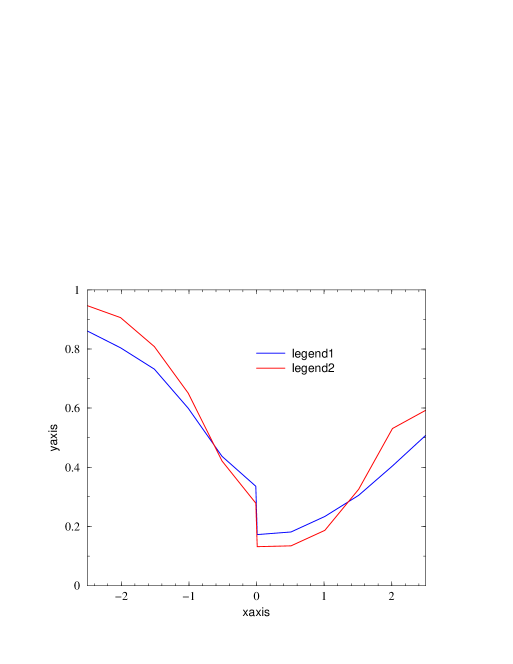
Figure 4: Average exceedance correlation functions between all pair of stocks as a function of the level parameter $\theta$, both for real data and the surrogate non Gaussian one-factor model.

References

-
[1]
Lillo F and R N Mantegna, 2000
Variety and Volatility in Financial Markets
Physical Review E 62, pages 6126-6134 -
[2]
Cizeau P, M Potters and J-P Bouchaud, 2001
Correlation structure of extreme stock returns
Quantitative Finance 1, pages 217-222 -
[3]
Lillo F and R N Mantegna, 2000
Symmetry alteration of ensemble return distribution in crash and rally days of financial market
European Physical Journal B 15, pages 603-606 -
[4]
F. Longin, B. Solnik, 2001
Extreme Correlation of International Equity Markets, Journal of Finance 56, pages 649-676