Polymers in long-range-correlated disorder

Abstract

We study the scaling properties of polymers in a $d$–dimensional medium with quenched defects that have power law correlations $\sim r^{-a}$ for large separations $r$. This type of disorder is known to be relevant for magnetic phase transitions. We find strong evidence that this is true also for the polymer case. Applying the field-theoretical renormalization group approach we perform calculations both in a double expansion in $\varepsilon=4-d$ and $\delta=4-a$ up to the 1-loop order and secondly in a fixed dimension ($d=3$) approach up to the 2-loop approximation for different fixed values of the correlation parameter, $2\leq a\leq 3$. In the latter case the numerical results need appropriate resummation. We find that the asymptotic behavior of self-avoiding walks in three dimensions and long-range-correlated disorder is governed by a set of separate exponents. In particular, we give estimates for the $\nu$ and $\gamma$ exponents as well as for the correction-to-scaling exponent $\omega$. The latter exponent is also calculated for the general $m$-vector model with $m=1,2,3$.

I INTRODUCTION

The influence of structural disorder on the critical behavior of various kinds of condensed matter remains one of the central problems in physics. In this paper, we are interested in the scaling laws that govern the behavior of polymers in disordered media when the defects are correlated or belong to some porous or sponge-like structure. Our main question of interest will be: does a small amount of correlated quenched structural defects in the medium induce changes to the universal properties of a polymer macromolecule?

It is well established that the universal scaling properties of long flexible polymer chains in a good solvent are perfectly described within a model of self-avoiding walks (SAWs) on a regular lattice desCloizeaux90 . The limit of SAWs with an infinite number of steps may be mapped to a formal $m\rightarrow 0$ limit of the $m$-vector model at its critical point deGennes79 . In particular, for the average square end-to-end distance $R_{e}$ and the number of configurations $Z_{N}$ of a SAW with $N$ steps on a regular lattice one finds in the asymptotic limit $N\to\infty$:

$$\langle R_{e}^{2}\rangle\sim N^{2\nu},\mbox{\hskip 30.00005pt}Z_{N}\sim z^{N}N^{\gamma-1}$$ (1)

where $\nu$ and $\gamma$ are the universal correlation length and susceptibility exponents for the $m=0$ model that only depend on the space dimensionality $d$ and $z$ is a non-universal fugacity. For $d=3$ the exponents read Guida $\nu=0.5882\pm 0.0011$ and $\gamma=1.1596\pm 0.0020$; whereas for $d=2$ exact values $\nu=3/4$ and $\gamma=43/32$ are known d2 .

The problem of SAWs on randomly diluted lattices, which may serve as a model of linear polymers in a porous medium, has been the subject of intensive discussion Chakrabarti ; Kim ; Harris83 ; Meir ; Grassberger93 ; Barat ; randomsaws ; Ordemann ; Blavats'ka01 . A recent review on SAW statistics on random lattices is given in ref. Barat . The numerical results for these systems available from Monte-Carlo simulations, exact enumeration and analytical treatment also cover the non-universal properties. Nonetheless, even apart from the numerical values of scaling exponents the question if a given form of disorder affects the scaling behavior has not been settled in general.

A frequently studied type of random lattice is the lattice that is diluted to the percolation threshold Barat . Here, one is interested in the behavior of a SAW on the percolation cluster. Scaling laws (1) hold with exponents that differ from their counter parts on a regular lattice at $d=2$ and $d=3$ Meir ; Grassberger93 . Apparently, this results from the fact that the percolation cluster itself is characterized by a fractal dimension which differs from $d$, the Euclidean one. Moreover, the scaling of the averaged moments of $Z_{N}$ (1) on the backbone of a percolation cluster possesses multifractal behavior Ordemann . In our study, however, we address another type of disorder, when the lattice is well above the percolation threshold. In this case the dimension of the support does not change and it is not clear a priori whether the SAW asymptotic exponents (1) will be influenced.

We approach this question for the case of long-range-correlated disorder using the connection between the scaling properties of polymers and magnets. So let us first turn our attention to the magnetic problem. While it is intuitively clear that strong disorder destroys the magnetic ordering, a much more subtle question is what happens at weak dilution by a non-magnetic component, i.e. well above the percolation threshold (weak disorder) Folk00 . It has been argued Harris that the presence of a non-correlated (or short-range-correlated) quenched disorder has a nontrivial effect on the critical behavior of magnetic systems, only if the specific heat critical exponent $\alpha$ of the pure magnet is positive. This statement is often called the Harris criterion. However, one should be careful in applying this “naively” to the SAW problem. Indeed, although the critical exponent $\alpha$ of a SAW on the $d=3$ dimensional pure lattice is positive Guida ($\alpha(d=3)=0.235\pm 0.003$), a weak quenched short-range-correlated disorder does not alter the SAW critical exponents. This statement has been proven by Harris Harris83 and confirmed later by renormalization group results Kim .

Note, that in the works mentioned above only uncorrelated quenched defects were investigated. In 1980-ies the model of a disordered $d$-dimensional system with so-called “extended” structural defects Cardy ; Dorogovtsev was developed. These defects are considered as quenched and correlated in a subspace of $\varepsilon_{d}$ dimensions, and randomly distributed in the remaining $d-\varepsilon_{d}$ dimensions. This model may be applied for small densities of defects. The integer values of $\varepsilon_{d}$ have a direct physical interpretation: $\varepsilon_{d}=0$ corresponds to short-range-correlated point-like defects, and the cases $\varepsilon_{d}=1,2$ are related, respectively, to lines and planes of impurities. To give an interpretation to non-integer values of $\varepsilon_{d}$, one may consider patterns of extended defects like aggregation clusters, and treat $\varepsilon_{d}$ as the fractal dimension of these clusters Yamazaki88 . In this interpretation the defect patterns are fractal, while the support of the system is the complement of this fractal and will in general not be fractal itself. In ref. Cardy the critical behavior of $O(m)$ symmetric magnets with extended defects with parallel orientation was investigated evaluating the renormalization group equations by a double $\varepsilon=4-d,\varepsilon_{d}$ expansion. It was found that the scaling is affected by these kinds of defects and the critical exponents were calculated in this scheme. The static and dynamic critical properties of $m$-component cubic-anisotropic systems with extended-defects were studied in the refs. Yamazaki using a double $\varepsilon,\varepsilon^{\prime}=\varepsilon+\varepsilon_{d}$-expansion again finding a change of critical behavior when $\varepsilon_{d}$ is increased.

In further work Weinrib attention concentrated on disordered systems with “random-temperature” disorder, arising from a small density of impurities that cause random variations in the local transition temperature $T_{c}(\vec{x})$. The fluctuations in $T_{c}(\vec{x})$ are characterized by a correlation function, that falls off according to a power law: $\sim x^{-a}$ at large distances $x$. It was shown, that in the presence of long-range-correlated disorder the Harris criterion is modified: for $a<d$ the disorder is relevant, if the correlation length critical exponent of the pure system obeys $\nu<2/a$. An $m$-vector model of this type was evaluated using a renormalization group expansion in the parameters $\varepsilon=4-d,\delta=4-a$ up to the linear approximation. An additional renormalization group fixed point corresponding to the long-range correlated disorder was found. In the following we will denote this as the ‘LR’ fixed point. The correlation-length exponent was evaluated in this linear approximation as $\nu=2/a$ and it was argued, that this scaling relation is exact and also holds in higher order approximation. However, this result was questioned recently in refs. Prudnikov , where the static and dynamic properties of 3d systems with long-range-correlated disorder were studied in a renormalization group approach using a 2-loop approximation. There is an essential discrepancy between the latter results and those found from the $\varepsilon,\delta$-expansion. Nevertheless it was qualitatively confirmed by both approaches that long-range-correlated disorder leads to a new universality class for these magnetic systems. Note, that the variable $a$ is a global parameter: together with the space dimension $d$ and the number of components $m$ of the order parameter it fixes the universal values of the critical exponents.

While the influence of long-range-correlated disorder on the magnetic phase transition has been the subject of considerable interest, the effect of long-range-correlated disorder on the scaling properties of polymers remains unclear and is generally not considered as settled. Here, we address the question of the asymptotic behavior of polymers in long-range-correlated disorder with algebraically decaying correlations Weinrib . While the linear approximation of the double $\varepsilon,\delta$-expansion indicates qualitatively the existence of the LR fixed point for polymers, it leads to unphysical quantitative results Blavats'ka01 . For this reason we present here an analysis of the 2-loop approximation using the fixed $a,d$-technique that leads to physically meaningful results for the scaling behavior of polymers in the LR regime.

Our paper is organized as follows: in the following section II we present the model, in section III the renormalization procedure is discussed and we reproduce the results of the $\varepsilon,\delta$-expansion. In section IV we apply resummation techniques to analyse the renormalization group functions in the two-loop approximation and find that the asymptotic behavior of self-avoiding walks in a three-dimensional medium with long-range-correlated disorder is governed by a new set of exponents. For the exponents we present quantitative estimates. Section V concludes our study. Some additional information about the properties of magnetic phase transitions in systems with long-range-correlated quenched disorder is presented in the appendix.

II THE MODEL

To study the universal properties of polymers in porous media with long-range-correlated quenched structural defects, we turn our attention to the investigation of the appropriate $m$-vector model in the polymer limit. We consider the model of an $m$-vector magnet, that is described by the following Hamiltonian:

$${\cal H}=\int d^{d}x\left[\frac{1}{2}\left((\mu_{0}+\delta\mu_{0}(x))\vec{\phi}^{2}+(\vec{\nabla}\vec{\phi})^{2}\right)+\frac{u_{0}}{4!}(\vec{\phi}^{2})^{2}\right],$$ (2)

here, $\vec{\phi}$ is an $m$-component field: $\vec{\phi}=\{\phi^{1}\cdots\phi^{m}\}$, $\mu_{0}$ and $u_{0}$ are the bare mass and the coupling of the undiluted magnetic model, $\delta\mu_{0}(x)$ represents the quenched random-temperature disorder, with:

$$\langle\langle\delta\mu_{0}(x)\rangle\rangle=0,$$

$$\frac{1}{8}\langle\langle\delta\mu_{0}(x)\delta\mu_{0}(y)\rangle\rangle=g(|x-y|),$$

where $\langle\langle\cdots\rangle\rangle$ denotes an average over spatially homogeneous and isotropic quenched disorder. The form of the pair correlation function $g(r)$ is chosen to fall off with distance according to a power law Weinrib :

$$g(r)\sim r^{-a}$$ (3)

for large $r$, where $a$ is a constant.

We consider quenched disorder and average the free energy over different configurations of the disorder. To this end we apply the replica method and construct an effective Hamiltonian for the $m$-vector model with long-range-correlated disorder Weinrib :

$${\cal H}_{\rm eff} = \sum_{\alpha=1}^{n}\int{\rm d}^{d}x\Big{[}\frac{1}{2}\left(\mu_{0}\vec{\phi}_{\alpha}^{2}+(\vec{\nabla}\vec{\phi}_{\alpha})^{2}\right)+\frac{u_{0}}{4!}(\vec{\phi}_{\alpha}^{2})^{2}\Big{]}{}-\sum_{\alpha,\beta=1}^{n}\int{\rm d}^{d}x{\rm d}^{d}yg(|x-y|)\vec{\phi}_{\alpha}^{2}(x)\vec{\phi}_{\beta}^{2}(y).$$ (4)

Here, the replica interaction vertex $g(r)$ is the correlation function given in Eq. (3), Greek indices denote replicas and the replica limit $n\to 0$ is implied.

For small $k$ the Fourier-transform $\tilde{g}(k)$ of $g(r)$ reads:

$$\tilde{g}(k)\sim v_{0}+w_{0}|k|^{a-d}.$$ (5)

Note, that in the case of random uncorrelated point-like defects the site-occupation correlation function formally reads: $g(|x-y|)\sim\delta(|x-y|),$ and its Fourier transform obeys:

$$\tilde{g}(k)\sim v_{0}.$$ (6)

Comparing Eqs. (5) and (6), it is obvious that the case $g(r)\sim r^{-d}$ corresponds to random uncorrelated point-like disorder. Moreover, different integer values of $a$ correspond to uncorrelated extended impurities of random orientations. So, the correlation function in Eq. (3) with $a=d-1$ describes straight lines of impurities of random orientation whereas random planes of impurities correspond Cardy to $a=d-2$. In terms of the fractal interpretation given in the introduction, the general case corresponds to SAWs on the complement of a fractal with dimension $\epsilon_{d}=d-a$.

Writing Eq. (4) in momentum space and taking Eq. (5) into account, one obtains an effective Hamiltonian with three bare couplings $u_{0},v_{0},w_{0}$. For $a>d$ the $w_{0}$-term is irrelevant in the renormalization group sense and one obtains the effective Hamiltonian of the quenched diluted (uncorrelated) $m$-vector model Grinstein with two couplings $u_{0},v_{0}$. For $a<d$ we have, in addition to the momentum-independent couplings, the momentum dependent one $w_{0}k^{a-d}$. Note that $\tilde{g}(k)$ must be positive being the Fourier image of the correlation function. This implies $w_{0}\geq 0$ for small $k$. Also the coupling $u_{0}$ must be positive, otherwise the pure system would undergo a first order phase transition.

The critical behavior of the model in Eq. (4) with $m\geq 1$ has been investigated Weinrib ; Prudnikov ; Elka using the renormalization group approach rgbooks . We are interested in the polymer limit $m\rightarrow 0$ of this model interpreting it as a model for polymers in a disordered medium. Note, that this limit is not trivial. For the case $u_{0}\neq 0,v_{0}\neq 0,w_{0}=0$ the “naive” RG analysis leads to controversial results about the absence of a stable fixed point and thus to the absence of the second order phase transition Chakrabarti . As noticed by Kim Kim , once the limit $m,n\to 0$ has been taken, the $u_{0}$ and $v_{0}$ terms are of the same symmetry, and an effective Hamiltonian with one coupling of $O(mn=0)$ symmetry results. This leads to the conclusion that weak quenched uncorrelated disorder is irrelevant for polymers as long as $v_{0}<u_{0}$.

Our present analysis takes these symmetry properties into account. In the case of the Hamiltonian with a term for long-range-correlated disorder Eq. (4) we pass to an effective Hamiltonian Blavats'ka01 with only two couplings $U_{0}=u_{0}-v_{0}$ and $w_{0}$ (in what follows below we will keep the notation $u_{0}$ for this new coupling $U_{0}$). In discrete momentum space this effective Hamiltonian reads:

$${\cal H}_{\rm eff} = \sum_{k}\sum_{\alpha}^{n}\frac{1}{2}(\mu_{0}+k^{2})(\vec{\phi}_{k}^{\alpha})^{2}+\frac{u_{0}}{4!}\sum_{\alpha}^{n}\sum_{k_{1}k_{2}k_{3}k_{4}}\delta(k_{1}+k_{2}+k_{3}+k_{4})\left(\vec{\phi}_{k_{1}}^{\alpha}\vec{\phi}_{k_{2}}^{\alpha}\right)\left(\vec{\phi}_{k_{3}}^{\alpha}\vec{\phi}_{k_{4}}^{\alpha}\right)-$$

$$\frac{w_{0}}{4!}\sum_{\alpha\beta}^{n}\sum_{kk_{1}k_{2}k_{3}k_{4}}|k|^{a-d}\delta(k_{1}+k_{2}+k)\delta(k_{3}+k_{4}-k)\left(\vec{\phi}_{k_{1}}^{\alpha}\vec{\phi}_{k_{2}}^{\alpha}\right)\left(\vec{\phi}_{k_{3}}^{\beta}\vec{\phi}_{k_{4}}^{\beta}\right),\quad m,n\rightarrow 0.$$

Here, the $\delta(k)$ represent products of Kronecker symbols and the notation $\left(\vec{\phi}\vec{\phi}\right)$ implies a scalar product. Note that the $w_{0}$-term itroduces interactions between the replicas and contains the power of an internal momentum. Again, it may be shown that for $a=d$ in the limit $m,n\rightarrow 0$ the $u_{0}$ and $w_{0}$ terms are of the same symmetry and one is left with an $O(mn=0)$-vector model with only one coupling $(u_{0}-w_{0})$.

III THE RENORMALIZATION

In order to extract the critical behavior of the model, we use the field-theoretical renormalization group (RG) method. We choose the massive field theory scheme with renormalization at non-zero mass and zero external momenta Parisi that leads to Callan-Symanzik equations for the renormalized one-particle irreducible vertex functions $\Gamma^{(M)}_{R}$. In our case the renormalization conditions Prudnikov are written both in fixed $d$ and $a$. The renormalized mass $\mu$ and renormalized couplings $u,w$ are defined by:

$$\mu^{2} = \Gamma_{R}^{(2)}(k,\mu^{2},u,w)|_{k=0},$$

$$\mu^{4-d}u = \Gamma_{R,u}^{(4)}(\{k\},\mu^{2},u,w)|_{k=0},$$

$$\mu^{4-a}w = \Gamma_{R,w}^{(4)}(\{k\},\mu^{2},u,w)|_{k=0}.$$

Here, $\Gamma^{(4)}_{R,u}$ and $\Gamma^{(4)}_{R,w}$ are the contributions to the four-point vertex function $\Gamma^{(4)}_{R}$ that correspond to $u$- and $w$-term symmetry, respectively. Asymptotically close to the critical point the $M$-point renormalized vertex functions obey the homogeneous Callan-Symanzik equation rgbooks :

$$\left\{\mu\frac{\partial}{\partial\mu}+\sum_{i}\beta_{v_{i}}(\{v_{j}\})\frac{\partial}{\partial v_{i}}-\frac{M}{2}\gamma_{\phi}(\{v_{j}\})\right\}\Gamma^{(M)}_{R}(\{k\},\mu^{2},\{v_{j}\})=0,$$ (8)

here, $v_{i}=u,w$. The change of the couplings $u,w$ under renormalization defines a flow in parametric space that is governed by the corresponding $\beta$-functions $\beta_{u}(u,w)$, $\beta_{w}(u,w)$. The fixed points $u^{\ast},w^{\ast}$ of this flow are given by the solutions of the system of equations: $\beta_{u}(u^{\ast},w^{\ast})=0,\,\beta_{w}(u^{\ast},w^{\ast})=0.$ The stable fixed point is defined as the fixed point where the stability matrix:

$$B_{ij}=\frac{\partial\beta_{v_{i}}}{\partial v_{j}},$$ (9)

possesses eigenvalues $\omega_{i}$ with positive real parts. The accessible stable fixed point corresponds to the critical point of the system. The fixed point is accessible if it can be reached along flow lines starting from allowed initial values $u_{0},w_{0}\geq 0$. At the fixed point we define the correlation length and pair correlation function critical exponents $\nu$ and $\eta$ by

$$\nu^{-1} = 2-\gamma_{\phi}(u^{\ast},w^{\ast})-\gamma_{\phi^{2}}(u^{\ast},w^{\ast}),$$ (10)

$$\eta = \gamma_{\phi}(u^{\ast},w^{\ast}),$$ (11)

where $\gamma_{\phi^{2}}$ is the exponent that corresponds to the two-point vertex function $M=2$ with a $\phi^{2}$ insertion. Other critical exponents may be obtained from familiar scaling laws. For example, for the susceptibility exponent $\gamma$ one has:

$$\gamma=\nu(2-\eta).$$ (12)

According to the RG prescriptions given above, the RG functions are obtained in form of a series in the renormalized couplings. In the one-loop approximation the result reads Blavats'ka01 :

$$\beta_{u}=-\varepsilon\left[u-\frac{4}{3}\,u^{2}I_{1}\right]-\delta 2uw\left[I_{2}+\frac{1}{3}I_{4}\right]+(2\delta-\varepsilon)\frac{2}{3}\,w^{2}I_{3},$$ (13)

$$\beta_{w}=-\delta\left[w+\frac{2}{3}\,w^{2}I_{2}\right]+\varepsilon\frac{2}{3}\left[wuI_{1}-w^{2}I_{4}\right],$$ (14)

$$\gamma_{\phi^{2}}=\varepsilon\frac{u}{3}\,I_{1}-\delta\,\frac{w}{3}\,I_{2},\phantom{55}\gamma_{\phi}=\delta\,\frac{w}{3}I_{4}.$$ (15)

Here, $I_{i}$ are one-loop integrals that depend on the space dimension $d$ and the parameter $a$:

$$I_{1}=\int\frac{{\rm d}\vec{q}}{(q^{2}+1)^{2}},\,\phantom{5}I_{2}=\int\frac{{\rm d}\vec{q}\,q^{a-d}}{(q^{2}+1)^{2}},\,\phantom{5}I_{3}=\int\frac{{\rm d}\vec{q},\,q^{2(a-d)}}{(q^{2}+1)^{2}}\,\phantom{5}I_{4}=\frac{\partial}{\partial k^{2}}\left[\int\frac{{\rm d}\vec{q}\,q^{a-d}}{[q+k]^{2}+1}\right]_{k^{2}=0}.$$ (16)

Note that contrary to the usual $\phi^{4}$ theory the $\gamma_{\phi}$ function in Eq. (15) is nonzero already in one-loop order. This is due to the $k$-dependence of the integral $I_{4}$ in Eq. (16).

There are two ways to proceed in order to obtain the qualitative characteristics of the critical behavior of the model. One can consider the polynomials in Eqs. (13), (14) for fixed $a,d$ and look for the solution of the fixed point equations. It is easy to check that these one-loop equations do not have any stable accessible fixed points for $d<4$. The other scheme to evaluate these equations is a double expansion in $\varepsilon=4-d$ and $\delta=4-a$ as proposed by Weinrib and Halperin Weinrib . Formerly Blavats'ka01 , we exploited this up to the linear approximation. For completeness, we here note those results. Substituting the loop integrals in Eqs. (13)-(15) by their expansion in $\varepsilon=4-d$ and $\delta=4-a$ , one obtains the 3 fixed points given in thea Table 1. We may draw the following conclusions from these first order results: Three distinct accessible fixed points are found to be stable in different regions of the $a,d$-plane. The Gaussian (G) fixed point, the pure (P) SAW fixed point and the long-range (LR) disorder SAW fixed point. The corresponding regions in the $a,d$-plane are marked by I, II and III in fig. 1. In the region IV no stable fixed point is accessible.

For the correlation length critical exponent of the SAW, one finds distinct values $\nu_{\rm pure}$ for the pure fixed point and $\nu_{\rm LR}$ for the long-range fixed point. Taking into account that the accessible values of the couplings are $u>0$, $w>0$, one finds that the long-range stable fixed point is accessible only for $\delta<\varepsilon<2\delta$, or $d<a<2+d/2$, a region where power counting in Eq. (II) shows that the disorder is irrelevant. In this sense the region III for the stability of the LR fixed point is unphysical. Formally, the first order results for $d<4$ read:

$$\nu=\left\{\begin{array}[]{ll}\nu_{\rm pure}=1/2+\varepsilon/16,&\delta<\varepsilon/2,\\ \nu_{\rm LR}=1/2+\delta/8,&\varepsilon/2<\delta<\varepsilon.\end{array}\right.$$ (17)

Thus, in this linear approximation the asymptotic behavior of polymers is governed by a distinct exponent $\nu_{\rm LR}$ in the region III of the parameter plane $a,d$ .

Something similar happens if the $\varepsilon,\delta$–expansion is applied to study models of $m$–vector magnets with long-range-correlated quenched disorder. For comparison, using the results of Weinrib and Halperin Weinrib we get the phase diagram presented for $m=2$ in the fig. 2. Although the critical behavior of the long-range-correlated universality class appears there for $a<d$ where it is relevant by power counting (region III in the fig. 2) this region in the $d-a$ plane is separated from the critical behavior of the $O(m=2)$ universality class by a region, where no accessible stable fixed points are present (IV in fig. 2). It means that also in the case of magnets, as well as for polymers the first order $\varepsilon,\delta$–expansion leads to a controversial phase diagram (compare figs. 1 and 2). So our first order results should be considered as purely qualitative and in order to obtain a clear picture and more reliable information, we proceed to higher order calculations.

IV THE RESUMMATION AND THE RESULTS

Fortunately, to investigate the 2-loop approximation in a fixed $d$ and $a$ approach we need not recalculate the intermediate expressions of perturbation theory for the vertex functions. Instead, we may make use of $m\to 0$ limit of the appropriate $m$-vector model, investigated recently Prudnikov . Starting from the two-loop expressions of ref. Prudnikov for the RG functions of the $m$-vector magnet with long-range-correlated disorder and applying the symmetry arguments Kim ; Blavats'ka01 for the polymer limit $m=0$ as explained in Section II we get the following expressions for the $d=3$ RG functions of the model in Eq. (II):

$$\beta_{u}(u,w) = -u+u^{2}-(3f_{1}(a)-f_{2}(a))uw-\frac{95}{216}u^{3}+\frac{1}{8}b_{2}(a)u^{2}w-$$ (18)

$$(b_{3}(a)+\frac{1}{4}b_{6}(a))uw^{2}+f_{3}(a)w^{2}+b_{5}(a)w^{3},$$

$$\beta_{w}(u,w)=-(4-a)w-(f_{1}(a)-f_{2}(a))w^{2}+\frac{uw}{2}+b_{10}(a)w^{3}-\frac{23}{216}u^{2}w+\frac{1}{4}b_{12}(a)uw^{2}$$ (19)

$$\gamma_{\phi}(u,w)=\frac{1}{2}f_{2}(a)w+\frac{1}{108}u^{2}+c_{1}(a)w^{2}-\frac{1}{4}c_{2}(a)uw,$$ (20)

$$\gamma_{\phi^{2}}(u,w)=\frac{1}{4}u-\frac{1}{2}f_{1}(a)w-\frac{1}{16}u^{2}-c_{3}(a)w^{2}+\frac{1}{4}c_{4}(a)uw.$$ (21)

Here, the coefficients $f_{i}(a)$ are expressed in terms of the one-loop integrals in Eq. (16), $b_{i}(a)$ and $c_{i}(a)$ originate from two-loop integrals and are tabulated in ref. Prudnikov for $d=3$ and different values of the parameter $a$ in the range $2\leq a\leq 3$. The series are normalized by a standard change of variables $u\to\frac{3u}{4}I_{1},w\to\frac{3w}{4}I_{1}$, so that the coefficients of the terms $u,u^{2}$ in $\beta_{u}$ become $1$ in modulus.

The RG functions listed above have the form of a divergent series, with zero radius of convergence Hardy , familiar to the theory of critical phenomena rgbooks . If the nature of the divergence is such that the series are asymptotic, then the situation is, at least in principle, controllable: in this case a good estimate for the sum of the series is obtained by keeping a certain number of the first terms (“optimal truncation”) or applying an appropriate resummation procedure.

For the case of the pure 3-dimensional $\phi^{4}$ theory it is known that the perturbation series are asymptotic, and Borel-summability in 3 dimensions has been proven Eckmann . The situation of the random-site Ising model is less satisfactory than for the pure system Folk00 . For instance, the asymptotic parameter in the disordered system is $\sqrt{\varepsilon}$ instead of $\varepsilon$, and the $\beta$-functions, computed at two loops show no stable fixed points. Bray et al Bray and McKane McKane studied the asymptotic expansion for the free energy of the random-site Ising model in the zero-dimensional case, and the model was found to be non-Borel summable. However, recently Alvarez the Borel summability of the perturbation expansion for the zero-dimensional disordered Ising model was proven analytically, provided that the summation is carried out in two steps: first, in the coupling of the pure Ising model and subsequently in the variance of the quenched disorder.

In our case, the summability of the series in Eq. (18) is open. Nevertheless, we apply various kinds of resummation techniques note1 , in order to obtain reliable quantitative results for the problem under consideration and to check the stability of these results.

IV.1 Chisholm-Borel resummation

First, we employ a simple two-variable Chisholm-Borel resummation technique Jug . For our problem this turns out to be the most effective one. The resummation procedure consists of several steps:

(i) starting from the initial RG function $f$ in the form of a truncated series note1 in the variables $u$ and $w$, one constructs its Borel image:

$$f=\sum_{i,j}a_{ij}u^{i}w^{j}\rightarrow\sum_{i,j}\frac{a_{ij}(ut)^{i}(wt)^{j}}{\Gamma(i+j+1)},$$

where $\Gamma(x)$ is the Euler’s gamma function;

(ii) the Borel image is extrapolated by a rational Chisholm Chisholm ; Baker approximant $[K/L](ut,wt)$ which is defined as the ratio of two polynomials both in the variables $u$ and $w$ of degrees $K$ and $L$ such that the truncated Taylor expansion of the approximant is equal to that of the Borel image of the function $f$;

(iii) the resummed function $f^{\rm res}$ is then calculated as the inverse Borel transform of this approximant:

$$f^{\rm res}=\int\limits_{0}^{\infty}{\rm d}t\exp(-t)[K/L](ut,wt).$$

There are a lot of possibilities to choose a Chisholm approximant in two variables. The most natural way is to construct it such that, if any of $u$ or $w$ is equal to zero, it leads to the familiar results for the reduced model. Here, for the Borel-images of the $\beta$-functions Eqs. (18), (19) we have chosen the following approximants with linear denominators:

$$\beta_{u}(u,w,t)^{\rm chis}=\frac{a_{1,0}ut+a_{2,0}u^{2}t^{2}+a_{1,1}uwt^{2}+a_{0,2}w^{2}t^{2}+a_{2,1}u^{2}wt^{3}+a_{1,2}uw^{2}t^{3}}{1+b_{1,0}ut+b_{0,1}wt},$$

$$\beta_{w}(u,w,t)^{\rm chis}=\frac{c_{0,1}wt+c_{0,2}w^{2}t^{2}+c_{2,1}u^{2}wt^{3}+c_{1,2}uw^{2}t^{3}}{1+d_{1,0}ut+d_{0,1}wt}.$$ (22)

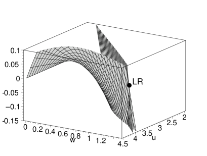
Figure 3: The Chisholm-Borel resummed 3d $\beta$-functions in the two-loop approximation at $a=2.9$. The flat surface corresponds to the $\beta_{w}$-function. The resummation restores the presence of a pure SAW fixed point $(u^{\ast}=1.63,w^{\ast}=0)$ and leads to a new stable “long-range-correlated” fixed point. The coordinate box is chosen to show the stable LR fixed point $(u^{\ast}=4.13,w^{\ast}=1.47)$ on the face of the box.

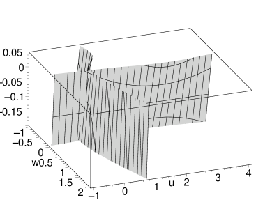
Figure 4: The non-resummed 3d $\beta$-functions at $a=2.9$. The intersection of the $\beta_{u}$ and $\beta_{w}$ surfaces with the $u-w$ plane give the fixed points. Only the Gaussian fixed point $u^{\ast}=w^{\ast}=0$ is present without resummation.

Note, that the polynomials in the numerators are chosen to be symmetric in the variables $u,w$. In fig. 3 we show the resummed 3d $\beta$-functions in the $u,w$-plane for $a=2.9$. In addition to the familiar fixed points describing Gaussian chains and polymers we obtain the stable LR fixed point for polymers in long-range-correlated disorder. For comparison, we depict the nonresummed functions in fig. 4. Only the Gaussian fixed point ($u^{*}=0,w^{*}=0$) is obtained without resummation. In figure 5 we visualize the situation depicting the lines of zeroes of the resummed $\beta$-functions at $a=2.9$ in the $u,w$-plane in the region of interest. The intersections of these curves correspond to the fixed points. The corresponding values of the stable fixed point coordinates and the stability matrix eigenvalues for different values of the correlation parameter $a<3$ are given in our Table 2.

Substituting Eqs. (20), (21) into Eqs.(10)–(12) we get the following expressions:

$$\nu^{-1}(u,w) = 2-\frac{1}{4}u+\frac{(f_{1}(a)-f_{2}(a))}{2}w+\frac{(c_{2}(a)-c_{4}(a))}{4}uw+\frac{23}{432}u^{2}+(c_{3}(a)-c_{1}(a))w^{2},$$

$$\gamma(u,w) = 1+\frac{1}{8}u-\frac{f_{1}(a)}{4}w+\frac{(f_{2}(a)+4c_{4}(a)-2f_{1}(a))}{32}uw-\frac{1}{64}u^{2}+$$ (23)

$$\frac{(f_{1}^{2}(a)-f_{1}(a)f_{2}(a)-8c_{3}(a))}{16}w^{2}.$$

This defines the critical exponents by $\nu^{-1}=\nu^{-1}(u^{*},w^{*})$ and $\gamma=\gamma(u^{*},w^{*})$ at the stable accessible fixed point ($u^{*},w^{*}$). To calculate these exponents in the region where the LR fixed point is stable, we again perform a resummation of the series in Eq. (23), using the following Chisholm approximants:

$$\frac{c_{0,0}+c_{0,1}wt+c_{1,0}ut+c_{1,1}uwt^{2}}{1+d_{1,0}ut+d_{0,1}wt}.$$ (24)

The critical exponent $\eta$ is obtained from the scaling law in Eq. (12). The numerical values for $\nu$, $\gamma$ and $\eta$ are listed in Table 2 for $a=2.3,\dots,2.9$. Note, that for $a=3$, which corresponds to short-range-correlated point-like defects, the interactions $u$ and $w$ become of the same symmetry, so we pass to one coupling $(u-w)$ and reproduce the well-known values of the critical exponents for the pure SAW model. The numerical values corresponding to those listed in table 2 are in this case: $u^{*}=1.63$, $\nu=0.59$, $\gamma=1.17$, $\eta=0.02$, $\omega=0.64$. As departing from the value $a=3$ downward to $2$ one notices a major increase of the value of the coupling $u$, so the results are more reliable for $a$ close to 3. At some value $a=a_{\rm marg}$ the LR fixed point becomes unstable. This is explained by the following physical interpretation: as noted in the introduction, the case $a=d-1$ (in our 3d approach $a=2$) corresponds to straight lines of impurities of random orientation, and the absence of stable fixed points for $a$ near $a=2$ suggests the collapse of the polymer chain in such a medium.

It is difficult to estimate the accuracy of the numerical values presented in Table 2. On one hand, it is the first non-trivial result: in the one-loop approximation at fixed $d$, $a$ one does not encounter the LR fixed point so one can not estimate deviations caused by different orders of the perturbation theory. On the other hand, as is known from the experience with the studies of magnets with long-range-correlated disorder Prudnikov , the convergence of the resummed series for the RG functions is worse than in the pure (or the short-range-correlated) case. The resummed two-loop expansions we exploited here give quite reliable estimates for the exponents of SAWs on the pure ($d=3$) lattice (compare our two-loop values $\nu=0.59$ and $\gamma=1.17$ with the most precise RG estimates cited just after Eq. (1)). In the case of the short-range-correlated diluted magnets the comparison of recent six-loop results Pelissetto with the two-loop ones Jug brings about the accuracy of latter of the order of several percents. While for our case no higher order calculations are available to test the numerical accuracy of the data in Table 2 the results clearly confirm the presence of a new stable fixed point LR with critical exponents that differ from those of the “pure” fixed point P.

In order to confirm the quantitative stability of the picture we obtained, we have also used different non-symmetric approximants for $\beta_{w}$ instead of the one given in Eq. (22). As expected, this approach was less effective in the sense that the region where a stable fixed point could be established was reduced and the numerical values differed from those given in Table 2. Nonetheless, the qualitative picture is the same: an LR fixed point exists and is stable in some interval $a_{\rm marg}\leq a<3$.

IV.2 Subsequent resummation

Secondly, we applied the method of subsequent resummation, developed in the context of the $d=0$ dimensional diluted Ising model in ref. Alvarez and successfully used for the $d=3$ case in ref Pelissetto . Here, the summation was carried out first in the coupling $u$ and subsequently in $w$. Starting from the $\beta$-functions in Eqs. (18), (19) we rewrite them as series in the variable $w$:

$$\beta_{u}(u,w) = -u+u^{2}-\frac{95}{216}u^{3}+w\left(u(f_{2}(a)-3f_{1}(a))+\frac{b_{2}}{8}u^{2}\right)$$

$$+w^{2}\left(f_{3}(a)-u(b_{3}(a)+\frac{b_{6}(a)}{4})\right)+b_{5}(a)w^{3},$$

$$\beta_{w}(u,w) = w\left(a-4+\frac{u}{2}-\frac{23}{216}u^{2}\right)+w^{2}\left(f_{2}(a)-f_{1}(a)+\frac{b_{12}(a)}{4}u\right)+b_{10}(a)w^{3}.$$

We first perform a Padé-Borel resummation of the coefficients at different powers of $w$ in the variable $u$, where it is possible. This results in a series of the form:

$$f(u,w)=\sum_{i}A_{i}(u)w^{i}.$$ (25)

The coefficients $A_{i}$ are some functions of $u$. Finally, the series (25) are resummed in the variable $w$. While we do not expect any high accuracy from this method, as far as the applicability has not been proven for our problem, again the presence of a stable fixed point LR for $a_{\rm marg}\leq a<d$ in this case confirms the stability of a new type of critical behavior.

We note that in addition to the above procedures we have tried a Padé-Borel approximation for the summation of the RG functions. To treat the two variable case we used the representation in terms of a resolvent series Watson ; Baker in a single auxiliary variable. However, no fixed points with $w\neq 0$ were found in the region of interest. But note, that even for the weakly diluted quenched Ising model this procedure does not lead to stable fixed points in the three loop approximation Folk00 .

IV.3 Interpretation of the numerical results

We may summarize and interpret our results as follows:

(i) A new stable fixed point (LR) for polymers in long-range-correlated disorder is found for $d=3$, $a<d$, leading to critical exponents that are different from those of the pure model;

(ii) There is a marginal value $a_{\rm marg}$ for the parameter $a$, below which the stable fixed point is absent, indicating a chain collapse of the polymer for disorder that is stronger correlated.

(iii) The critical exponent $\nu$ increases with decreasing parameter $a$, like in the Weinrib and Halperin case. But note, that the relation $\nu=2/a$ does not hold. Physically this means that in weak long-range-correlated disorder ($a>a_{\rm marg}$) the polymer coil swells with increasing correlation of the disorder. The self avoiding path of the polymer has to take larger deviations to avoid the defects of the medium.

V CONCLUSIONS

In the present work, we have analysed the scaling behavior of polymers in media with quenched defects that are correlated with a correlation that decays like $\sim 1/x^{a}$ for large separations $x$. This type of disorder is known to be relevant in magnetic systems Weinrib ; Prudnikov , but the question about its relevance in the polymer problem was so far not answered. To this end we applied the field-theoretical RG approach, and performed renormalization for fixed mass and zero external momenta Parisi . In our study we take special care of the symmetry properties of the effective Hamiltonian of the system Kim . Formerly Blavats'ka01 we performed calculations up to the linear approximation, using a double $\varepsilon,\delta$-expansion, as proposed for the magnetic problem in the work of Weinrib and Halperin Weinrib . While already this study indicated the possibility of a new type of critical behavior in such a system, it predicted such behavior for an unphysical range of parameters. A more sophisticated investigation at higher order of the perturbation series was needed to confirm the existence of a distinct polymer scaling behavior for long range correlated disorder.

We use 2-loop expressions for the RG functions that were recently obtained for $m$-component systems in the fixed $d,a$ approach Prudnikov and apply appropriate resummation techniques. This way we confirm that in a medium with long-range-correlated quenched disorder the swelling of the polymer coil is governed by a distinct exponent $\nu_{\rm LR}$ that increases when the correlation of the disorder is increased (i.e. $a$ is decreased). When the correlation is too strong, i.e. $a$ is below some marginal value $a_{\rm marg}>\approx 2$, then a crossover to the collapse of the polymer is predicted.

VI Appendix

Here, we turn our attention to the 3d magnetic system. Recently Ballesteros and Parisi Ballesteros presented Monte-Carlo simulations of the site-diluted Ising model in three dimensions in the presence of quenched disorder with long-range-correlations. The values of the corrections-to-scaling exponents are of great interest in the interpretation of such simulations. In previous work, dedicated to 3d magnets with long-range-correlated disorder Prudnikov ; Dorogovtsev ; Cardy these exponents have not been calculated. Here we carry out these calculations based on the $\beta$-functions of the model Eq. (4) in the 2-loop approximation, as presented in ref. Prudnikov .

The correction-to-scaling exponent is defined as the minimal stability matrix eigenvalue in the stable accessible fixed point. We carry out the investigation in new variables $(u,v,w)\to(u,v,v+w)$, as proposed by Dorogovtsev Dorogovtsev and perform the Padé-Borel resummation of the $\beta$-functions. The results are presented in Table 3.

Fixed Point	$u^{\ast}$	$w^{\ast}$	$\omega_{1}$	$\omega_{2}$
Gaussian (G)	$0$	$0$	$-\varepsilon$	$-\delta$
Pure SAW (P)	$\varepsilon$	$0$	$\varepsilon$	$\varepsilon/2-\delta$
Long-range (LR)	$\frac{2\delta^{2}}{(\varepsilon-\delta)}$	$-\frac{\delta(\varepsilon-2\delta)}{(\varepsilon-\delta)}$	$\phantom{555555}\frac{1}{2}\{\varepsilon-4\delta\pm\sqrt{\varepsilon^{2}-4\varepsilon\delta+8\delta^{2}}\}$

Table 1: Fixed points and stability matrix eigenvalues in the first order of the $\varepsilon,\delta$ - expansion.

$a$	$u^{*}$	$w^{*}$	$\nu$	$\gamma$	$\eta$	$\omega_{1,2}$
2.9	4.13	1.47	0.64	1.25	0.04	0.25 $\pm$ 0.62 i
2.8	4.73	1.68	0.64	1.26	0.04	0.22 $\pm$ 0.76 i
2.7	5.31	1.81	0.65	1.28	0.03	0.18 $\pm$ 0.89 i
2.6	5.89	1.87	0.66	1.29	0.03	0.15 $\pm$ 0.99 i
2.5	6.48	1.89	0.66	1.31	0.02	0.11 $\pm$ 1.09 i
2.4	7.10	1.87	0.67	1.33	0.01	0.07 $\pm$ 1.18 i
2.3	7.76	1.84	0.68	1.36	0.01	0.03 $\pm$ 1.26 i

Table 2: Stable fixed point of the 3d two-loop $\beta$-functions, resummed by the Chisholm-Borel method, the corresponding critical exponents and the stability matrix eigenvalues at various values of $a$.

$a$	2	2.1	2.2	2.3	2.4	2.5	2.6	2.7	2.8	2.9
$\omega(m=1)$	0.80	0.81	0.83	0.87	0.94	1.14	1.07	0.87	0.71	0.69
$\omega(m=2)$	1.15	1.08	0.93	0.86	0.81	0.68	0.59	0.57	0.55	0.54
$\omega(m=3)$	0.88	0.83	0.76	0.67	0.62	0.61	0.60	0.60	0.59	0.68

Table 3: The correction-to-scaling exponents $\omega$ for the phase transition in the 3d $m$-vector model with $m=1,2,3$.

Figure 1: The critical behavior of a polymer in a medium with long-range-correlated disorder in different regions of the $d,a$-plane as predicted by the first order $\varepsilon,\delta$–expansion. Region I corresponds to the Gaussian random walk behavior, in the region II scaling behavior is the same as in the medium without disorder, in region III the “long-range” fixed point LR is stable and the scaling laws for polymers are altered, in region IV no accessible stable fixed points appear; this may be interpreted as the collapse of the chain.

Figure 2: The critical behavior of the $m=2$-magnet in a medium with long-range-correlated disorder in different regions of the $d,a$-plane as predicted by the first order $\varepsilon,\delta$–expansion. Region I corresponds to the mean field behavior, in the region II the critical exponents are the same as in the medium with uncorrelated disorder, in III the fixed point LR is stable, in IV no accessible stable fixed points appear.

Figure 5: The lines of zeroes of the 3d $\beta$-functions (18), (19) resummed by the Chisholm-Borel method at $a=2.9$. The dashed line corresponds to $\beta_{u}=0$, the solid lines depict $\beta_{w}=0$. The intersections of the dashed and solid lines give three fixed points shown by filled circles at $u^{\ast}=0,w^{\ast}=0$ (G), $u^{\ast}=1.63,w^{\ast}=0$ (P), and $u^{\ast}=4.13,w^{\ast}=1.47$ (LR). The fixed point LR is stable.

References

- (1) J. des Cloizeaux, G. Jannink, Polymers in Solution. (Clarendon Press, Oxford, 1990); L. Schäfer L, Universal Properties of Polymer Solutions as Explained by the Renormalization Group (Springer, Berlin, 1999).
- (2) P.-G. de Gennes, Scaling Concepts in Polymer Physics (Cornell University Press, Ithaca and London, 1979).
- (3) Recent renormalization group estimates for critical exponents are found in: R. Guida, J. Zinn Justin. J. Phys. A 31, 8104 (1998).
- (4) B. Nienhuis, Phys. Rev. Lett. 49, 1062 (1982); P. Grassberger, Z. Phys. B 48, 255 (1982).
- (5) B. K. Chakrabarti and J. Kertész, Z. Phys. B – Condensed Matter 44, 221 (1981).
- (6) Y. Kim, J. Phys. C 16, 1345 (1983).
- (7) A.B. Harris, Z. Phys. B 49, 347 (1983).
- (8) Y. Meir and A. B. Harris, Phys. Rev. Lett. 63, 2819 (1989).
- (9) P. Grassberger, J. Phys. A 26, 1023 (1993).
- (10) K. Barat and B. K. Chakrabarti, Phys. Reports 258, 377 (1995).
- (11) S. B. Lee and H. Nakanishi, Phys. Rev. Lett. 61, 2022 (1988); S. B. Lee, H. Nakanishi and Y. Kim, Phys. Rev. B 39, 9561 (1989); J. Machta and T.R. Kirkpatrick, Phys. Rev. A 41, 5345 (1990); A.V. Izyumov and K. B. Samokhin, J. Phys. A 32, 7843 (1999); A. R. Altenberger, I. I. Siepmann, and J. S. Dahler, J. Phys. A 272, 22 (1999); Y. Shiferaw and Y.Y. Goldschmidt, J. Phys. A 33, 4461 (2000).
- (12) For recent references see e.g. A. Ordemann, M. Porto, H. E. Roman, S. Havlin, and A. Bunde, Phys. Rev. E 61, 6858 (2000); A. Ordemann, M. Porto, H. E. Roman, and S. Havlin, Phys. Rev. E 63, 0104 (2001).
- (13) V. Blavats’ka, C. von Ferber, and Yu. Holovatch, J. Mol. Liq. 91, 77 (2001).
- (14) About an influence of a non-correlated weak quenched disorder on a magnetic phase transition see e.g. R. Folk, Yu. Holovatch, and T. Yavorsk’ii, Phys. Rev. B 61, 15114 (2000) for a recent review.
- (15) A.B. Harris, J. Phys. C 7, 1671 (1974).
- (16) D. Boyanovsky and J. L. Cardy, Phys. Rev. B 26, 154 (1982).
- (17) S.N. Dorogovtsev, J. Phys. A 17, 677 (1984).
- (18) Y. Yamazaki, A. Holz, M. Ochiai, and Y. Fukuda, Physica A 150, 576 (1988).
- (19) Y. Yamazaki, A. Holz, M. Ochiai, and Y. Fukuda, Phys. Rev. B 33, 3460 (1985); Y. Yamazaki, Y. Fukuda, A. Holz, and M. Ochiai, Physica A 136, 303 (1986).
- (20) A. Weinrib and B.I. Halperin, Phys. Rev. B 27, 413 (1983).
- (21) V.V. Prudnikov, P.V. Prudnikov, and A.A. Fedorenko, J. Phys. A 32, L399 (1999); V.V. Prudnikov, P.V. Prudnikov, and A.A. Fedorenko, J. Phys. A 32, 8587 (1999); V.V. Prudnikov, P.V. Prudnikov, and A.A. Fedorenko, Phys. Rev. B 62, 8777 (2000).
- (22) G. Grinstein and A. Luther, Phys. Rev. B, 13, 1329 (1976).
- (23) E. Korutcheva and F. Javier de la Rubia, Phys. Rev. B 58, 5153 (1998).
- (24) E. Brézin, Le Guillou J C, Zinn-Justin J, ”Field theoretical approach to critical phenomena” in Phase Transitions and Critical Phenomena, edited by C. Domb and M. S. Green, Vol. 6, Academic Press, London, 1976; D. J. Amit, Field Theory, the Renormalization Group, and Critical Phenomena (World Scientific, Singapore, 1989); J. Zinn-Justin, Quantum Field Theory and Critical Phenomena (Oxford University Press, 1996); H. Kleinert, V. Schulte-Frohlinde, Critical Properties of -Theories (World Scientific, Singapore, 2001).
- (25) Parisi G., in Proceedings of the Cargèse Summer School, 1973, (unpublished); J. Stat. Phys. 23, 49 (1980).
- (26) G. H. Hardy, Divergent Series (Oxford, 1948).
- (27) J. P. Eckmann, J. Magnen, and R. Sénéor, Commun. Math. Phys. 39, 251 (1975).
- (28) A. J. Bray, T. McCarthy, M. A. Moore, J. D. Reger, and A. P. Young, Phys. Rev. B 36, 2212 (1987).
- (29) A. J. McKane, Phys. Rev. B 49, 12 003 (1994).
- (30) G. Álvarez, V. Martín-Mayor, and J. J. Ruiz-Lorenzo, J. Phys. A 33, 841 (2000).
- (31) G. Jug, Phys. Rev. B, 27, 609 (1983).
- (32) J. S. R. Chisholm, Math. Comp. 27, 841 (1973).
- (33) G. A. Baker, Jn. and P. Graves-Morris, Padé Approximants (Addison-Wesley, Reading, MA, 1981).
- (34) We perform our analysis of the two-loop expressions for the RG functions in the fixed technique. It is known that for other models with disorder, the -expansion leads to less reliable results Folk00 .
- (35) A. Pelissetto and E. Vicari, Phys. Rev. B 62, 6393 (2000).
- (36) P. J. S. Watson, J. Phys. A 7, L167 (1974).
- (37) H. G. Ballesteros and G. Parisi, Phys. Rev. B 60, 12912 (1999).